Figures & data
Figure 1. Example of TEOAEs measured in one ear using the double-evoked paradigm, evoked using a high-pass filtered click stimulus with a stimulus level of 75 dB peSPL. Each trace shows two replicates (one black, one grey) overlaid. The top trace shows the overall signal. The lower eight traces show the output from the ½-octave filter banks, with the centre frequency shown at the right end of each trace. The time-window over which the TEOAE is analysed is shown by vertical dashed lines. A scale bar is shown on the left-hand side as a thick black line.
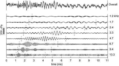
Figure 2. Box and whisker plots the TEOAEs and HTLs across conventional and extended high-frequency regions. Boxes represent the interquartile range, with the median shown by a horizontal line. Circles indicate minor outliers, defined using fences 1.5 times the interquartile range. Whiskers represent the maximum and minimum values excluding outliers. (A) shows TEOAE amplitudes in ½-octave bands. Grey boxplots indicate centre frequencies used in calculating the EHF-TEOAE amplitude (i.e. 9.4 and 13.3 kHz); white boxplots indicate octave bands from 1.2 to 6.7 kHz which are used for descriptive purposes only. The TEOAEs at centre frequencies from 6.7 to 13.3 kHz denoted “HPF” were obtained using the high-pass filtered click stimulus; the other TEOAEs were those obtained using a conventional click stimulus. (B) shows the SNR of TEOAEs corresponding to the measurements described for (A). (C) shows the HTL at 10 frequencies; the grey boxplots indicate those values used to calculate the 6-frequency average EHF HTL, while the white boxes indicate the HTLs shown for descriptive purposes only.
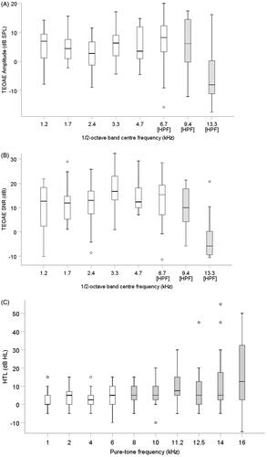
Figure 3. Example of two replicates of the Bekesy audiometry track for one participant (grey line: replicate 1; black line: replicate 2). (A) shows the total HTL-vs-frequency function. (B) shows the audiogram coarse structure obtained by the smoothing the trace in (A) using a moving-average filter with an averaging window in the logarithmic frequency domain coresponindg to 12.5% frequency interval (C) shows the audiogram fine-structure (AFS) obtained from the difference between the traces in (A,B). (D) show the reciprocal spectral periodicity distribution, obtained from of the Fourier series coefficients of the total HTL-vs-log frequency in (A). The values on the horizontal axis in (D) are equivalent to values of fC/Δf.
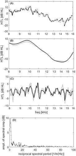
Figure 4. An example of the average AFS of the two replicates with turning points extracted.
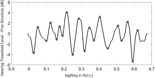
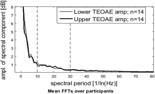
Figure 5. The reciprocal spectral periodicity distribution averaged across individuals. Averages from two subgroups of the sample are plotted separately. Grey line is for the subgroup, n = 14 with the highest EHF TEOAEs averages. The black line is for the subgroup, n = 14 with lowest EHF TEOAEs averages.