Test-retest evaluation of a notched-noise test using consumer-grade mobile audio equipment

Figures & data

Figure 1. Two spectra of a noise band (0.01–10 kHz) with a spectral notch of ±0.2 kHz around 2 kHz, presented via the two different playback systems after compensating for differences in frequency responses by inverse filtering.

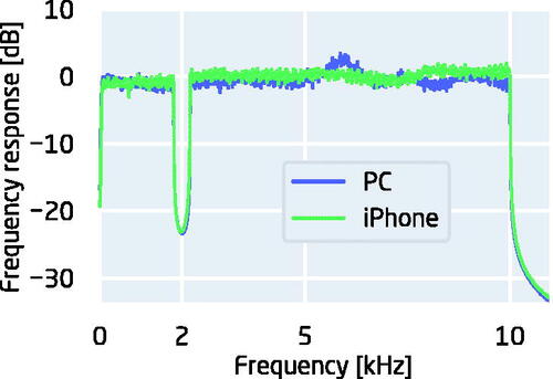
Figure 2. Illustration of one run of the grid method. The track starts with a moderately high signal level at zero notch width. Level is decreased until the signal detection threshold ($L_{\mathit{sig}}^{\mathit{th}}(\Delta ),$ shown as a grey line) is reached, after which the notch is increased until there is again a correct response.

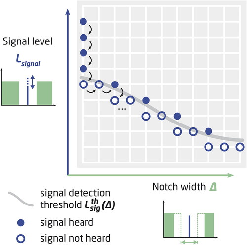
Figure 3. Detection thresholds as a function of notch width for Study 1. Thin lines show the individual threshold curves. The round and triangular symbols are the same in all figures and show data from Rosen and Baker (1994) and Weber (1977), respectively.

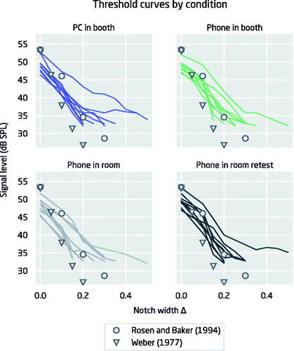
Figure 4. Pairwise Bland–Altman plots visualising test–retest repeatability for tone–in–noise-thresholds (threshold at zero notch) between two conditions in Study 1. The horizontal line shows the average difference in thresholds between two conditions, and the shaded area illustrates the 95% limits of agreement (mean ±1.96 SD) between the two conditions. The vertical grey dashed lines show the tone–in–noise-thresholds from Rosen and Baker (1994) and Weber (1977).

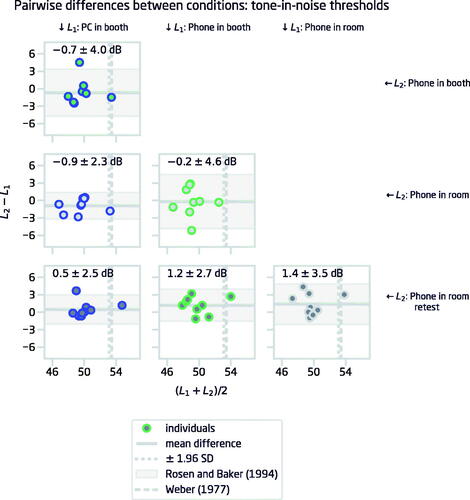
Figure 5. Pairwise Bland–Altman plots visualising test–retest repeatability for the p parameter of the roex filter in Study 1. The horizontal line shows the average difference in p, and the shaded area illustrates the 95% limits of agreement (mean ± 1.96 SD) between the two conditions.

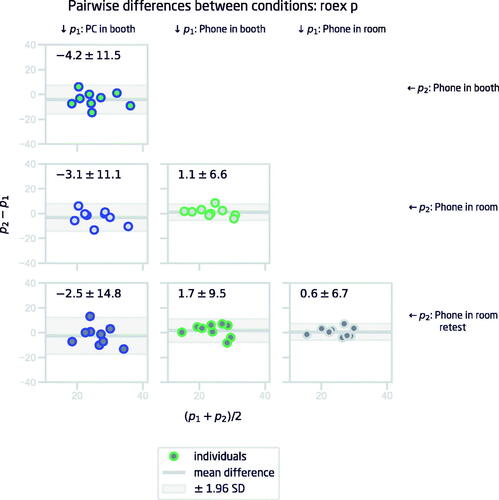
Table 1. The mean (standard deviation) of the p parameter and the corresponding equivalent rectangular bandwidth (erb) of the roex filter for each condition of Study 1.

Condition	p	r/dB	k/dB	erb/Hz
PC in booth	27.4 (6.9)	−72 (33)	−4.6 (2.6)	309 (78)
Phone in booth	23.2 (6.1)	−106 (50)	−4.8 (2.4)	366 (99)
Phone in room	24.3 (5.0)	−90 (40)	−5.6 (1.8)	343 (77)
Phone in room retest	24.9 (5.1)	−98 (50)	−4.1 (2.0)	336 (85)

Figure 6. Detection thresholds as a function of notch width for Study 2. The thin lines show the individual threshold curves. The round and triangular symbols are the same in all figures and show data from Rosen and Baker (1994) and Weber (1977), respectively.

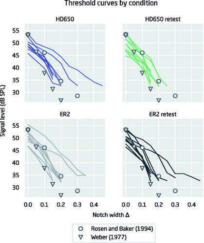
Figure 7. Pairwise Bland–Altman plots visualising test–retest repeatability for tone–in–noise-thresholds (threshold at zero notch) between the two conditions in Study 2. The horizontal line shows the average difference in thresholds between two conditions, and the shaded area illustrates the 95% limits of agreement (mean ±1.96 SD) between the two conditions. The vertical grey dashed lines show the tone–in–noise-thresholds from Rosen and Baker (1994) and Weber (1977).

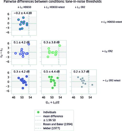
Figure 8. Pairwise Bland–Altman plots visualising test–retest repeatability for the p parameter of the roex filter in Study 2. Horizontal line shows the average difference in p, and the shaded area illustrates the 95% limits of agreement (mean ± 1.96 SD) between the two conditions.

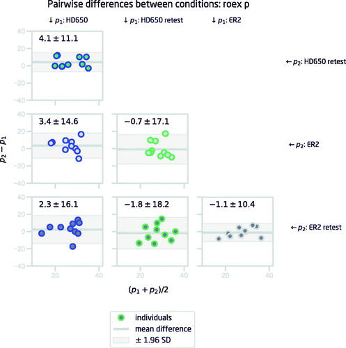
Table 2. The mean (standard deviation) of the p parameter and the corresponding equivalent rectangular bandwidth (erb) of the roex filter for each condition of Study 2.

condition	p	r/dB	k/dB	erb/Hz
HD650	24.6 (6.9)	−124 (33)	−4.9 (1.8)	351 (108)
HD650 retest	28.7 (6.5)	−102 (31)	−3.8 (3.1)	291 (65)
ER2	28.0 (5.4)	−129 (40)	−2.8 (3.0)	294 (53)
ER2 retest	27.0 (7.7)	−111 (52)	−3.9 (2.9)	327 (125)

Rosen, S., and R. J. Baker. 1994. “Characterising Auditory Filter Nonlinearity.” Hearing Research 73 (2): 231–243. doi:10.1016/0378-5955(94)90239-9

 PubMed Web of Science ®Google Scholar

Weber, D. L. 1977. “Growth of Masking and the Auditory Filter.” The Journal of the Acoustical Society of America 62 (2): 424–429. doi:10.1121/1.381542.

 PubMed Web of Science ®Google Scholar