Mapping collective human activity in an urban environment based on mobile phone data

Figures & data

Figure 1. City of Udine (Northern Italy); the grid size represents the spatial resolution (250 × 250 m²) of the mobile network traffic dataset used (the cells in the regular grid do not relate to the network antennas’ service areas.).

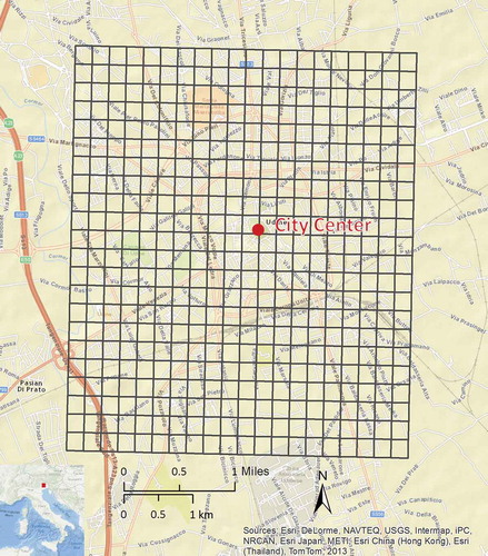
Table 1. Attribute matrix of the user-generated mobile phone data set used.

	Incoming	Outgoing
Voice calls	Number of calls terminated in a given grid cell but originating from another, adjacent cell	Number of calls originating from a given grid cell but terminated in another, adjacent cell
Text messages SMS	Number of text messages terminated in a given grid cell but originating from another, adjacent cell	Number of calls originating from a given grid cell but terminated in another, adjacent cell
Total traffic	The total network traffic is measured in Erlang and implicitly contains certain types of VGI and is therefore used as a proxy for the overall collective mobile communication activity; the total traffic refers to a given single cell

Figure 2. 3D visualization of mobile phone activity (categorized by received SMS, in (a); outgoing SMS, in (b); received phone call, in (c); placed phone call, in (d) and overall internet traffic in (e). The shaded envelope denotes 99% of the activity, the triangulated envelope 95%. Voxels are red-colored to reinforce the overall intensity.

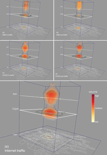
Figure 3. Overview of the Methodology: from raw mobile phone data (left) to spatiotemporal information on collective human activity (right).

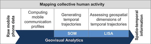
Figure 4. From multi-dimensional mobile communication profiles (sample input data) to temporal trajectories of change on the SOM output space.

Figure 5. Temporal trajectories on the SOM output space (regular point pattern): the location of nodes, which reflect similarity among the five variables, serve as vertices for the corresponding hour of the day (0–23); a, b and c show examples of trajectories with a similar length but different location/extent and shape/geometry, respectively.

Figure 6. Temporal trajectories in the SOM output space classified by their length on weekdays (top) and weekend (bottom); shortest trajectories in green on the left, longest in red on the right; the black ellipses denote visually outstanding trajectories within the same class (created with GeoTime Software).

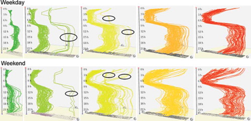
Figure 7. Spatial distribution of normalized trajectory lengths mapped in geographic space (left: typical weekend; right typical weekday); cells of visually outstanding trajectories from Figure 6 are highlighted.

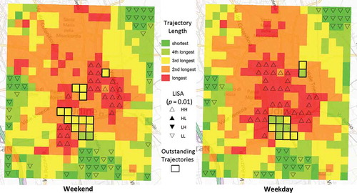
Table 2. Global Moran’s I summary on the trajectories’ total length.

	Typical weekday	Typical weekend
Moran’s index	0.713	0.688
Expected index	−0.002	−0.002
Variance	0.002	0.002
z-score	14.661	14.152
p-value	<0.01	<0.01

Figure 8. Spatiotemporal patterns of variations of collective human activity: weekend-weekday correlation and LISA of temporal changes in intensity and similarity mobile communication profiles per cell for 24 hours; the graph in each cell shows the normalized length of trajectories’ segments for each hour of the day; details a, b and c show examples of two spatial outliers and a cold-spot, as well as their corresponding locations on the grid (major streets are indicated as transparent white lines for orientation purposes).

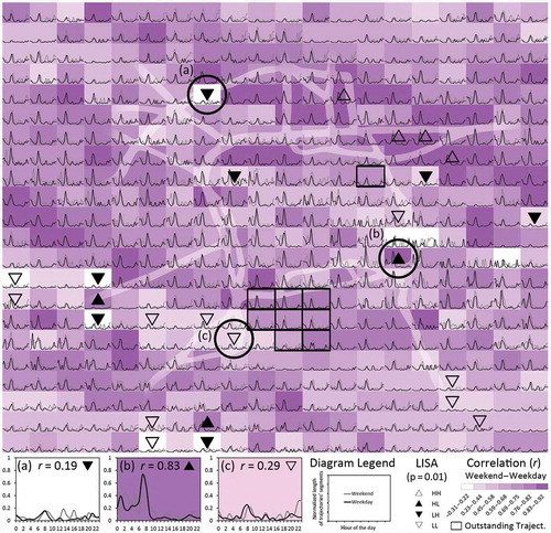
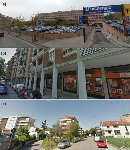
Figure 9. Virtual ground truthing: (a) several parking lots next to a hospital and medical university in the street “Via Forni di Sotto”; (b) multistoried buildings with both diverse businesses (ground floor) and apartments in the street “Viale Ungheria”; (c) urban residential area in the street “Via Palermo.”

Source: Google Street View, last accessed 16 August 2013.