Population downscaling using high-resolution, temporally-rich U.S. property data

Figures & data

Figure 1. Population density in 2000 by census tract in: a) Connecticut, b) South Carolina, c) Oregon, d) New Mexico. The barplot on the lower-left corner of each graph shows the number of census tracts by population density, with “L,” “M,” and “H” indicating low population density (< 250 persons/km²), medium population density (250 ~ 1,000 persons/km²), and high population density (>1,000 persons/km²) categories

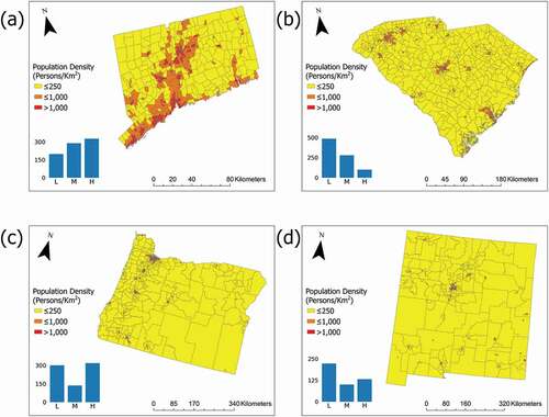
Table 1. Number of census tracts (CTs) with 0 BUPR in the four studied states

	Total number of CTs	Number of CTs with BUPR of zero	Percent of CTs with BUPR of zero
Connecticut	816	0	0%
New Mexico	456	90	19.7%
Oregon	755	6	0.8%
South Carolina	867	34	3.9%

Table 2. Accuracy assessment results for dasymetric mapping using different ancillary data sources. The ranks in Table 2 are based on the percentage of people placed incorrectly, though all three metrics produce similar rankings. Except for BUPR, accuracy assessment results based on ancillary data sources are directly obtained from Zandbergen and Ignizio (2010)

	People placed incorrectly
Technique	Count	Percentage	Rank	Median Abs. % error	R-squared
Connecticut
BUPR	232,910	7.0	1	9.8	0.780
Minor road density	351,506	10.6	2	17.9	0.664
Total road density	364,320	11.0	3	18.7	0.642
Impervious < 75%	374,961	11.3	4	18.8	0.618
Land cover	394,724	11.9	5	18.8	0.582
Impervious < 60%	407,589	12.3	6	20.2	0.589
Total impervious	408,770	12.4	7	19.7	0.561
Cleaned imperviousness	503,041	15.2	8	22.6	0.409
Nighttime lights	525,464	15.9	9	26.7	0.487
Areal weighting	559,739	16.9	10	27.9	0.447
New Mexico
Land cover	252,371	14.5	1	21.1	0.519
Impervious < 60%	282,282	16.2	2	21.8	0.411
Impervious < 75%	283,816	16.3	3	22.8	0.413
Total impervious	297,869	17.1	4	25.2	0.416
Cleaned imperviousness	306,141	17.5	5	26.3	0.415
BUPR	369,675	21.2	6	28.5	0.336
Nighttime lights	370,561	21.2	7	36.1	0.378
Minor road density	371,693	21.3	8	29.3	0.255
Total road density	378,025	21.6	9	31.9	0.254
Areal weighting	511,848	29.3	10	46.7	0.143
Oregon
BUPR	261,937	7.9	1	10.7	0.812
Impervious < 60%	442,384	13.4	2	20.8	0.631
Land cover	452,171	13.6	3	21.2	0.628
Impervious < 75%	478,797	14.5	4	23.1	0.596
Total impervious	496,891	15.0	5	23.4	0.572
Cleaned imperviousness	505,111	15.2	6	23.9	0.591
Minor road density	620,544	18.7	7	25.4	0.375
Total road density	624,702	18.9	8	25.8	0.376
Nighttime lights	660,438	19.9	9	32.1	0.394
Areal weighting	863,315	26.1	10	41.3	0.234
South Carolina
BUPR	457,296	11.8	1	14.93	0.620
Impervious < 75%	476,633	12.3	2	20.3	0.722
Land cover	512,542	13.3	3	22.5	0.679
Impervious < 60%	517,606	13.4	4	22.2	0.683
Minor road density	551,732	14.3	5	22.9	0.624
Total road density	568,710	14.7	6	23.8	0.607
Total impervious	596,205	15.4	7	25.7	0.609
Nighttime lights	628,932	16.3	8	27.2	0.578
Cleaned imperviousness	829,252	21.5	9	36.1	0.449
Areal weighting	859,254	22.3	10	38.1	0.377

Figure 2. Bar plot for the percent of people placed incorrectly for each technique in the four states.

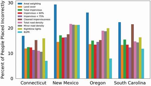
Table 3. Percentage of people placed incorrectly by population density category

	< 250 /km^2		250 to 1000/km^2		>1000/km^2
Technique	(%)	Rank	(%)	Rank	(%)	Rank
Connecticut	(n = 633) (m = 0%)		(n = 874) (m = 0%)		(n = 1057) (m = 0%)
BUPR	5.4	1	6.0	1	9.1	1
Minor road density	11.2	2	9.5	2	11.3	4
Total road density	11.3	3	10.2	3	11.6	7
Impervious < 60%	12.2	4	10.4	4	14.2	9
Land cover	12.7	5	12.2	6	11.2	3
Impervious < 75%	13.1	6	10.4	4	11.1	2
Total impervious	14.1	7	12.3	7	11.5	6
Nighttime lights	15.2	8	18.0	9	14.4	8
Areal weighting	18.3	9	18.5	10	17.3	10
Cleaned imperviousness	23.4	10	13.5	8	11.3	4
New Mexico	(n = 589) (m = 39%)		(n = 323) (m = 32%)		(n = 439) (m = 5%)
Land cover	19.0	1	12.3	3	9.2	3
Impervious < 75%	23.5	2	11.7	2	8.9	2
Cleaned imperviousness	23.5	2	15.4	6	10.2	5
Total impervious	23.6	4	13.3	4	10.1	4
Impervious < 60%	23.7	5	11.1	1	8.8	1
Nighttime lights	24.9	6	25.0	9	12.7	9
BUPR	27.6	7	21.7	8	11.1	8
Minor road density	31.9	8	15.1	5	10.2	5
Total road density	32.0	9	16.0	7	10.4	7
Areal weighting	40.1	10	29.0	10	13.3	10
Oregon	(n = 1049) (m = 2%)		(n = 426) (m = 0%)		(n = 976) (m = 0%)
BUPR	7.0	1	8.1	1	8.6	4
Land cover	17.8	2	15.0	5	9.4	5
Impervious < 60%	19.3	3	13.4	2	8.1	1
Total impervious	19.7	4	16.2	8	10.3	7
Impervious < 75%	20.1	5	13.6	3	9.8	6
Cleaned imperviousness	20.6	6	15.5	7	10.4	8
Nighttime lights	26.1	7	27.0	9	11.4	9
Total road density	32.4	8	15.2	6	8.5	3
Minor road density	32.7	9	14.6	4	8.3	2
Areal weighting	40.5	10	29.8	10	11.6	10
South Carolina	(n = 1691) (m = 3%)		(n = 849) (m = 5%)		(n = 258) (m = 3%)
BUPR	11.8	1	11.6	3	13.3	9
Impervious < 75%	13.0	2	11.5	2	10.4	2
Total impervious	15.4	5	16.0	7	13.0	6
Impervious < 60%	13.9	4	13.1	5	10.7	3
Land cover	13.5	3	13.2	6	11.7	5
Nighttime lights	16.3	6	17.1	8	13.2	7
Minor road density	16.5	7	10.9	1	10.1	1
Total road density	16.8	8	11.7	4	10.8	4
Cleaned imperviousness	24.7	9	17.1	8	13.2	7
Areal weighting	25.3	10	18.4	10	13.3	9

Sample size (n) is reported as the number of block groups included in the accuracy assessment calculation, while m denotes the percentage of block groups with zero BUPR value. Besides BUPR, accuracy assessment results based on ancillary data sources are directly obtained from Zandbergen and Ignizio (2010).

Figure 3. BUPR values for block groups in the city center and suburban areas of Hartford, Connecticut

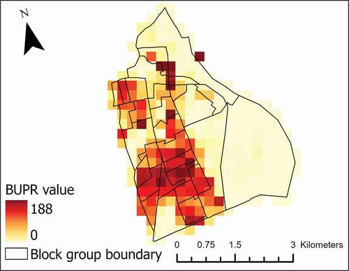
Figure 4. Scatter plot between block group areas and absolute error percentages generated from BUPR-based technique for the state of Connecticut. Both the areas and the absolute error percentages are log transformed to aid visualization (9 block groups out of a total of 2,555 with absolute error percentage values of 0 were removed as a log transformation is not applicable). The red dots denote the mean log absolute error percentage value for each log area category from −4 to 4 (incremented at an interval of 1). A secondary axis is also added to show the original values before log-transformation for easier interpretation

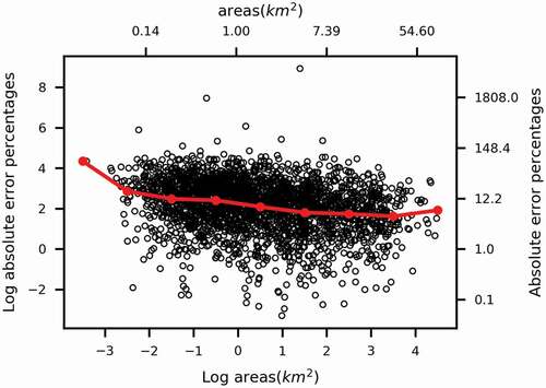
Figure 5. Kernel density plot for the block group areas (log transformed) in the four states. The red line indicates the value of a single BUPR pixel area (log transformed). Out of the 9,379 block groups, only 5 of them have an area smaller than the area of a single BUPR pixel (0.065 km²)

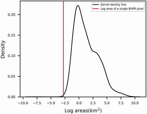
Figure 6. Error percentage between estimated and actual block group population in a) Connecticut; b) South Carolina; c) Oregon; d) New Mexico. Block groups with NA values indicate block groups with an actual population of 0

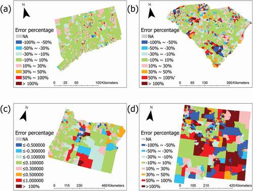
Figure 7. Mean absolute error percentage between downscaled population and actual population for each county across the contiguous United States

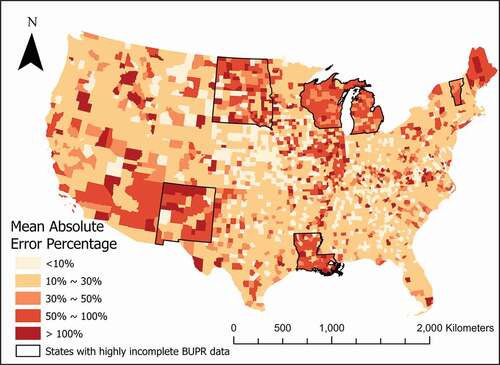
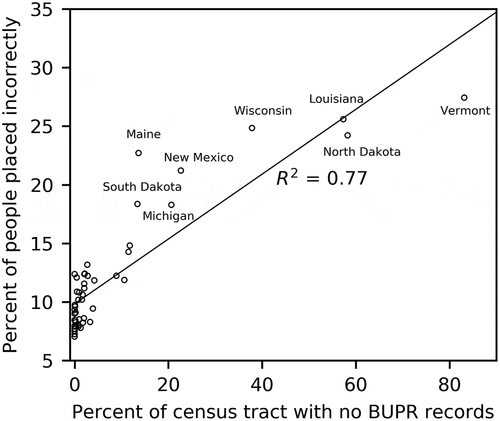
Figure 8. Scatter plot of the percentage of people placed incorrectly against the percentage of census tracts with no BUPR records for each state across the contiguous United States

Zandbergen, P. A., & Ignizio, D. A. (2010). Comparison of dasymetric mapping techniques for small-area population estimates. Cartography and Geographic Information Science, 37(3), 199–214. https://doi.org/https://doi.org/10.1559/152304010792194985

 Web of Science ®Google Scholar