Figures & data
Table 1. The type and time span of data sets used in individual analyses. Data are split by the focal question addressed, the variables examined, and the temporal extent of the data. For details, see Appendix,
Figure 1. Location of the Zackenberg camera rig, of the instrument measuring snow depth at the main climate mast, and of plots for monitoring arthropod and plant phenology in the Biobasis program (Schmidt et al. Citation2016a). A single orthorectified photograph from camera two (DoY 169 of 2014) is overlaid on the map under 10 m elevation contours
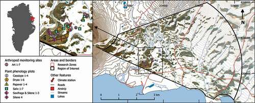
Figure 2. Temporal trends in (A) landscape level snowmelt date, as determined by 50 percent of land area uncovered, (B) maximum winter snow depth as measured at the snow depth mast next to the central climate station, and (C) above-zero degree days for spring and early summer (DoY ≥ 200)
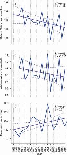
Figure 3. Variation in snowmelt dates (A) among sites and (B) among years within the Zackenberg valley. Panel (A) shows average day of year when the soil at a given site becomes exposed (scale on the right). Panel (B) shows interannual variability, expressed as the standard deviation of the timing of snowmelt (scale on the right). Both panels are based on nine years of data (2006–2014)
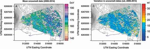
Figure 4. (A) Trend in the timing of snowmelt during 2006–2014 as a function of mean date of snowmelt for any given part (pixel) of the landscape. The average trend is negative, signaling that snowmelt is becoming earlier from year to year. Early melting pixels on average show a steeper trend than late melting sites (black trend line). (B) Scatter plot of average snowmelt pattern of individual pixels (i.e., typical earliness or lateness) and the consistency between mean snowmelt timing at the level of the pixel and the overall landscape (quantified by a correlation coefficient r). Most of the landscape follows the regional snowmelt pattern closely, with a correlation coefficient close to 1, with only a small share of all pixels diverging to a greater extent. Late sites (on the right of the x axis) show the largest variation
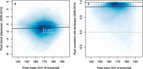
Figure 5. (A) Yearly snowmelt dates ± 1 standard deviation of the seven arthropod trapping sites situated at the bottom of the Zackenberg valley (see ). (B) Yearly snowmelt dates ± 1 standard deviation of plant phenology monitoring plots. The mean snowmelt date for the whole valley landscape is plotted for comparison (heavy grey line). Plots named as in Schmidt et al. (Citation2016a) and in
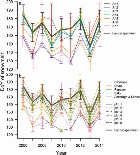
Figure 6. Relative proportions of variance in the phenology of plant and arthropod communities attributed to different factors. The variance attributed to the fixed effects is indicated by different shades of blue, whereas the variance attributed to random effects is indicated by different shades of yellow. The taxonomic categories match the original categories of the monitoring data, as here sorted by systematic position (order and class)
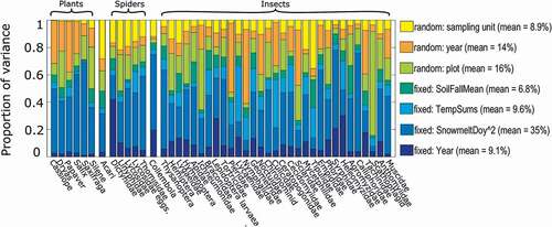
Table 2. Predicted phenological occurrences for groups of species with different dietary requirements
Table A1. Multiple linear regression model of snowmelt timing as a function of snow depth and spring temperatures
Table A2. Data sets used in the analyses included in this article
Table A3. Categories included as traits in the HMSC-analysis. For heterotrophs, the trait value describes adult diet, with "None" referring to typically nonfeeding adults. Flower feeders visit flowers for nectar or pollen resources
Figure A1. Validation of snowmelt data extracted from photographs as compared to ground-truthed observations. Shown are mean snowmelt dates measured from orthophotographs (x axis) and in situ observations of date of 50 percent snow cover (y axis) from the same arthropod and plant phenology plots. The latter includes some values with known uncertainties; that is, cases where the snow of the plot had melted before the first visit. The correlation coefficient (Pearson’s r) between the two is 0.88. The mean difference between mean snowmelt and 50 percent snow cover is 4.7 days