High-resolution ice sheet surface mass-balance and spatiotemporal runoff simulations: Kangerlussuaq, west Greenland

Figures & data

Figure 1. Kangerlussuaq simulation domain and catchment (12,825 km²; GrIS covered part 12,000 km²) with HydroFlow estimated drainage network and watershed divide between Sandflugtsdalen and Ørkendalen (dotted lines), 300-m contour interval, and locations for the K-transect AWSs S4–S9 and SHR (red dots). The inset figure (upper left) indicates the general location in Greenland. The inset figure (lower right) indicates a detailed illustration of the drainage system in the lower part of the catchment (below ~1,500 m a.s.l.), including the location of the Kangerlussuaq catchment outlet at the Watson River bridges (red square), outlet of Sandflugtsdalen (red triangle), and outlet from Ørkendalen (red diamond)

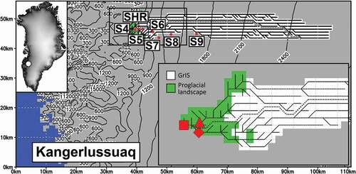
Figure 2. Kangerlussuaq GrIS catchment: (a) hypsometry, and (b) longitudinal elevation profile based on individual grids from the GrIS margin (west) to the highest elevated part of GrIS at the ice sheet divide (east). The locations of the K-transect stakes S4–S9 and SHR are shown

Table 1. Observed and SnowModel ERA-I simulated MAAT and standard deviation for the different K-transect AWS S5, S6, and S9 for variable observation periods and 1979–2014. Observed data from the AWS are operated by IMAU (van de Wal et al. 2005)

	S5	S6	S9
Observed (°C), period	−6.3 ± 8.2 (August 1993–August 2014)	−9.9 ± 8.3 (August 1995–August 2014)	−12.7 ± 8.6 (August 2003–August 2014)
Simulated (°C), period	−6.1 ± 9.3 (August 1993–August 2014)	−9.5 ± 8.5 (August 1995–August 2014)	−12.2 ± 8.2 (August 2003–August 2014)
Simulated (°C), 1979–2014	−6.7 ± 9.4	−9.4 ± 8.9	−12.3 ± 8.3

Table 2. Observed and SnowModel ERA-I simulated SMB mean and standard deviation for the different K-transect stakes S4–S9 and SHR for two periods 1990–2014 and 1979–2014. The value in the brackets illustrates the mean difference between observed and simulated SMB

	S4	S5	SHR	S6	S7	S8	S9	Mean
Observed 1990–2014 (m w.e yr^−1)	−4.15 ± 0.71	−3.68 ± 0.64	−3.08 ± 0.59	−1.66 ± 0.57	−1.48 ± 0.60	−0.78 ± 0.59	−0.12 ± 0.41	−2.14 ± 0.59
Simulated 1990–2014(m w.e yr^−1)	−3.83 ± 0.57	−3.56 ± 0.60	−3.21 ± 0.64	−2.24 ± 0.68	−1.94 ± 0.69	−1.08 ± 0.66	−0.32 ± 0.58	−2.31 ± 0.63 (0.17 ± 0.23)
Simulated 1979–2014(m w.e yr^−1)	−3.70 ± 0.56	−3.43 ± 0.58	−3.09 ± 0.62	−2.11 ± 0.66	−1.82 ± 0.67	−0.94 ± 0.65	−0.19 ± 0.55	−2.18 ± 0.61

Table 3. Observed and SnowModel ERA-I simulated mean Watson River outlet runoff and standard deviation for the years 2007–2013. Observed runoff is operated by GEUS (van As et al. 2012, 2017)

	2007	2008	2009	2010	2011	2012	2013	Mean
Observed discharge (m^3) (observed period)	7.51 × 10^9 (June 7–September 8)	5.46 × 10^9 (May 27–September 10)	4.87 × 10^9 (June 2–September 9)	11.24 × 10^9 (May 10–September 28)	7.77 × 10^9 (June 7–September 18)	10.73 × 10^9 (May 28–September 30)	4.32 × 10^9 (June 6–September 15)	7.41 × 10^9
Simulated discharge (m^3) (observed period)	11.65 × 10^9 (June 7–September 8) (63%)	8.04 × 10^9 (May 27–September 10) (66%)	6.67 × 10^9 (June 2–September 9) (69%)	13.66 × 10^9 (May 10–September 28) (82%)	11.68 × 10^9 (June 7–September 18) (66%)	14.97 × 10^9 (May 28–September 30) (71%)	8.22 × 10^9 (June 6–September 15) (52%)	10.69 × 10^9 (68 ± 9%)
Simulated discharge (m^3) (entire runoff period)	12.12 × 10^9	8.72 × 10^9	7.11 × 10^9	14.14 × 10^9	12.85 × 10^9	15.36 × 10^9	8.57 × 10^9	11.26 × 10^9
Adjusted simulated discharge (m^3) (entire runoff period)	7.67 × 10^9	5.75 × 10^9	4.89 × 10^9	11.53 × 10^9	8.54 × 10^9	10.94 × 10^9	4.45 × 10^9	7.69 × 10^9

Figure 3. SnowModel ERA-I simulated (1979–2014) and observed (1990–2014) SMB time series and scatter plots for the different K-transect stakes S4–S9 and SHR

Figure 4. Kangerlussuaq catchment observed and SnowModel ERA-I simulated daily discharge (2007–2013): (a) time series, (b) scatter plot, (c) adjusted discharge time series, and (d) adjusted discharge scatter plot

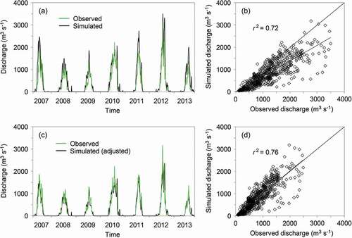
Figure 5. Kangerlussuaq GrIS catchment thirty-five-year mean daily SnowModel ERA-I simulated surface (1979–2014): (a) air temperature, (b) precipitation, (c) surface melt (snow and ice melt), (d) evaporation and sublimation, (e) ablation, and (f) SMB. The bold black line is the daily mean, the grey area indicates one standard deviation, and the red line indicates the year with the maximum accumulated value (for precipitation and SMB it is the yearly minimum accumulated values)

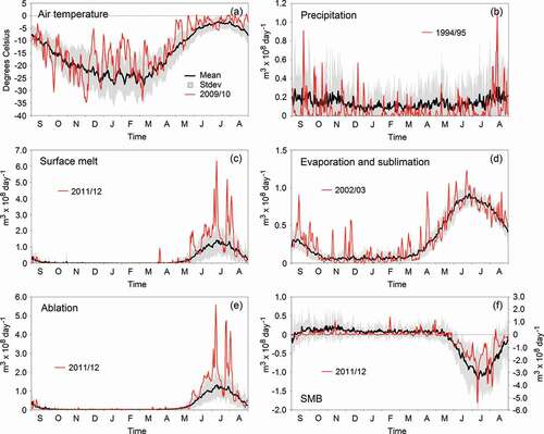
Figure 6. SnowModel ERA-I simulated time series of Kangerlussuaq GrIS catchment: (a) MAAT, (b) precipitation, (c) surface melt (snow and ice melt), (d) evaporation and sublimation, (e) ablation, and (f) SMB. Only significant trends are shown as linear fits through the data. For both (a) MAAT and (b) precipitation, ERA-I data are shown for the grid point located closest to the center of the Kangerlussuaq catchment (red time series). The grey shading is the ±10 percent (forced by a change in precipitation of ±10%). It is most visual for precipitation and SMB

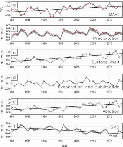
Figure 7. SnowModel ERA-I simulated thirty-five-year: (a) MAAT, (b) precipitation (snow and rain), (c) surface melt (snow and ice melt), (d) evaporation and sublimation, (e) ablation, and (f) SMB versus elevation

Figure 8. SnowModel ERA-I simulated thirty-five-year mean spatial Kangerlussuaq GrIS catchment surface (1979–2014): (a) MAAT, (b) precipitation, (c) surface melt (snow and ice melt), (d) evaporation and sublimation, (e) ablation, and (f) SMB

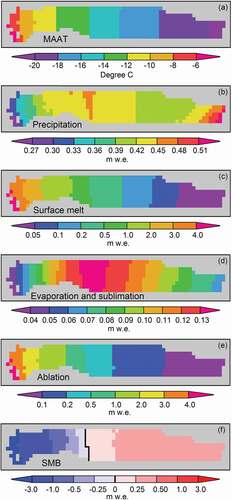
Figure 9. (a) SnowModel ERA-I time series of simulated daily Kangerlussuaq catchment outlet discharge from September 1979 to August 2014; (b) the origin and variability of annual runoff from rain, snowmelt, and ice melt; and (c) thirty-five-year mean runoff contributions (in percentage) from rain, snowmelt, and ice melt

Figure 10. SnowModel ERA-I simulated monthly mean runoff from rain, snowmelt, and ice melt for the runoff season May through October for 1979–2014, 1979–1984, and 2009–2014 for the outlet of Kangerlussuaq watershed

Figure 11. SnowModel ERA-I daily simulated discharge September 1979 through August 2014: (a) outlet of Sandflugtsdalen (6,800 km² and GrIS covered part 6,225 km² [92%], illustrated by a red triangle on Figure 1); (b) outlet of Ørkendalen (5,925 km² and GrIS covered part 5,775 km² [97%], illustrated by a red diamond on Figure 1); and (c) ratio between Sandflugtsdalen and Ørkendalen

Figure 12. SnowModel ERA-I simulated: (a) mean monthly runoff ratio between Sandflugtsdalen and Ørkendalen for the annual runoff period (May through October) for 1979–2014, 1979–1984, and 2009–2014, where the gray area equals one standard deviation; (b) time series of mean annual runoff ratio; and (c) the thirty-five-year mean runoff ratio

van de Wal, R. S. W., W. Greuell, M. R. van den Broeke, C. H. Reijmer, and J. Oerlemans. 2005. Surface mass-balance observations and automatic weather station data along a transect near Kangerlussuaq, West Greenland. Annals of Glaciology 42:311–16.

 Web of Science ®Google Scholar

van As, D., A. L. Hubbard, B. Hasholt, A. B. Mikkelsen, M. R. van den Broeke, and R. S. Fausto. 2012. Large surface meltwater discharge from the Kangerlussuaq sector of the Greenland ice sheet during the record-warm year 2010 explained by detailed energy balance observations. The Cryosphere 6:199–209.

 Web of Science ®Google Scholar

van As, D., A. B. Mikkelsen, M. H. Nielsen, J. E. Box, L. C. Liljedahl, K. Lindbäck, L. Pitcher, and B. Hasholt. 2017. Hypsometric amplification and routing moderation of Greenland ice sheet meltwater release. The Cryosphere 11:1371–1386. doi:https://doi.org/10.5194/tc-11-1371-2017.

 Google Scholar