The K-transect on the western Greenland Ice Sheet: Surface energy balance (2003–2016)

Figures & data

Figure 1. MODIS image of the Kangerlussuaq area, west Greenland. Automatic weather station (AWS) locations given as white circles. Photos demonstrate typical summer conditions at the four AWS locations

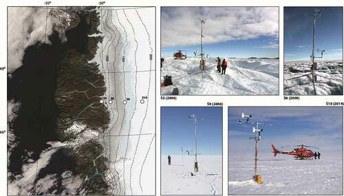
Table 1. Climatology at the automatic weather stations (AWS) locations for the period August 2003–August 2016. The wind directional constancy is calculated as the ratio of the magnitudes of the average vector and absolute wind speed (from Smeets et al. 2018)

Location	S5	S6	S9	S10
Height (m a.s.l.)	490	1020	1520	1850
Distance from ice edge (km)	6	38	88	140
Wind speed (m s^−1)	3.9	5.1	5.8
Temperature (°C)	−4.1	−8.5	−11.4
Relative humidity (%)	76	87	92
Specific humidity (g kg^−1)	2.1	1.9	1.6
Wind direction (°)	120	124	126
Directional constancy	0.87	0.91	0.82

Table 2. Sensor type and accuracy of observed variables for all automatic weather stations (AWS) (condensed from Smeets et al. 2018)

Variable	Sensor	Accuracy
Wind speed	05103-L.R.M. Young	0.3 m s^−1
Wind direction	05103-L.R.M. Young	3°
Temperature	Vaisala HMP45C	0.4°C at −20°C
Humidity	Vaisala HMP45C	2% for RH <90%
Net radiation	Kipp Zonen CNR1	10% of daily total
Pressure	Vaisala PTB101B	4 hPa
Surface height	height ranger SR50	0.01 m

Figure 2. Modeled versus observed surface temperature (°C, hourly values) for automatic weather station (AWS) locations (A) S5, (B) S6, (C) S9, and (D) S10. Mean bias dT and RMSE given in the lower right corner of each panel

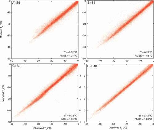
Figure 3. (A) Cumulative ice ablation in m w.e. for stations S5 and S6. Model data in solid lines (S5 in red, S6 in blue). Annual stake observations in squares (S5) and circles (S6). Note that modeled ablation for S6 was aligned to the stake data in September 2008, 2010, and 2012. (B) Annual ice ablation, model versus stake observations (in m w.e.) for S5 and S6

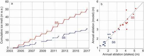
Figure 4. Monthly mean fluxes of net shortwave radiation (blue), net longwave radiation (red), sensible heat (orange), latent heat (green), ground heat (black), and melt (pink). From top to bottom: S5, S6, S9, and S10. The vertical axes are all at the same scale

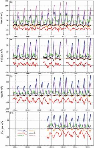
Figure 5. Hourly values of surface energy balance (SEB) fluxes (left vertical axis) and horizontal wind speed (right vertical axis) at S5 during a six-day period in August 2010

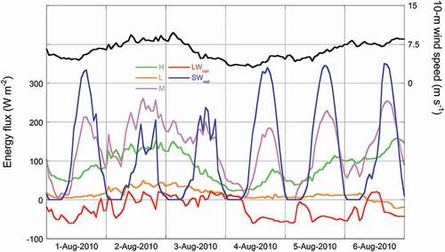
Table 3. Correlation coefficients (R) between June, July, August (JJA) mean melt flux and other surface energy balance (SEB) components

Correlation Coefficient with M	S5	S6	S9	S10
SWnet	0.57	0.78	0.88	0.79
LWnet	0.58	0.66	0.59	0.70
Rnet	0.86	0.98	0.98	0.93
H	0.78	0.74	0.71	0.29
L	0.88	0.78	0.60	0.46

Table 4. Trends in surface energy budget components, expressed in W m⁻² y⁻¹, determined for the period 2003–2016. Trends significant at the p < 0.10 level are shown in bold

Flux Trend (W m^−2 y^−1)		Hydrol. Year			JJA
	S5	S6	S9	S5	S6	S9
SWin	1.2	−0.1	0.8	3.8	0.5	2.4
SWout	0.4	−0.3	−0.6	1.7	−0.6	−1.3
SWnet	0.8	0.2	1.4	2.1	1.1	3.7
LWin	−1.1	−0.8	−0.6	−1.5	−1.0	−1.1
LWout	−0.7	−0.5	−0.1	−0.1	−0.2	0.0
LWnet	−0.4	−0.3	−0.5	−1.4	−0.9	−1.2
Rnet	0.4	−0.1	1.0	0.7	0.2	2.5
H	0.0	0.1	−0.1	0.1	0.1	0.0
L	−0.1	0.1	−0.2	−0.1	0.2	−0.2
M	0.0	−0.1	0.6	0.7	0.3	2.2

Figure 6. Energy fluxes (W m⁻²) averaged over June, July, August (JJA), sorted by JJA-mean melt flux. Years on horizontal axes

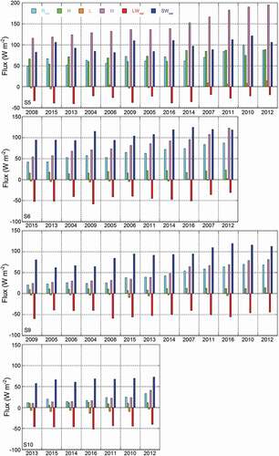
Figure 7. Mean June, July, August (JJA) albedo as a function of mean JJA melt flux (in W m⁻²). R² denotes the correlation coefficient

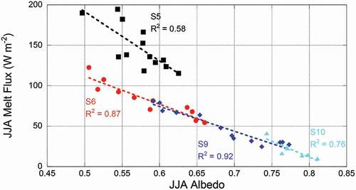
Figure 8. Total melt energy for each automatic weather stations (AWS) location, in MJ m⁻². June, July, August (JJA) totals in dashed lines with open circles. Annual totals in solid lines with closed circles. S5 in black, S6 in red, S9 in blue, and S10 in light blue

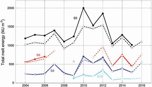
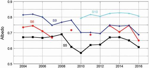
Figure 9. Albedo, computed from the mean incoming and reflected shortwave fluxes of each mass balance year (September 1, Y-1, to August 31, Y, where the year Y is given on the horizontal axis)

Smeets, C. J. P. P., P. Kuipers Munneke, M. R. van den Broeke, W. Boot, J. Oerlemans, H. Snellen, C. H. Reijmer, R. S. W. van de Wal, and D. van As. 2018. The K-transect in west Greenland: automatic weather station data (1993–2016). Arctic, Antarctic, and Alpine 50 (1):S100002.

 Google Scholar