The K-transect in west Greenland: Automatic weather station data (1993–2016)

Figures & data

Figure 1. Overview of the GIMEX91 experiment. AWS and SMB stakes were placed along an east–west running transect roughly perpendicular to the ice-sheet edge along the 67 N latitude line. UU/IMAU had a camp close to the ice edge (location 3, tethered balloon), while de FUA camp and boundary layer station, including a 31 m tower, were situated on the ice sheet (location S9). Location S10 was first established as an SMB site in August 1994. Blue represents the current SMB/GPS stations and red the current AWS sites

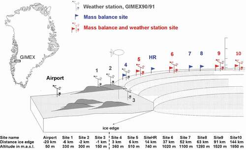
Table 1. Climatology at Kangerlussuaq (Kanger) and the AWS locations for the period from August 2003 to August 2016. The wind directional constancy is calculated as the ratio of the magnitudes of the average vector and absolute wind speed

Location	Kanger	S5	S6	S9	S10
Height (m asl)	50	490	1020	1520	1850
Distance from ice edge (km)	22	6	38	88	140
Wind speed u (ms^−1)	3.9	5.3	6.7	7.3	7.2
Temperature T (°C)	−3.9	−5.8	−10.2	−12.7	−15.6
Relative humidity RH (%)	65	77	87	90	92
Specific humidity q (gkg^−1)	2.8	2.4	2.2	2.0	1.8
Wind direction dd (°)	65	115	130	127	128
Directional constancy	0.56	0.89	0.89	0.85	0.68

Table 2. List of instruments used at UU/IMAU AWS Type I and Type II. The periods represent mass balance years, September 1 to August 31

Variable	Sensor type	Period	Accuracy	Sampling interval (minutes)
AWS Type I (1993–2001)
wind speed	Aanderaa 2740	1993–2001	0.5 ms^−1	6
wind direction	Aanderaa 2750	1993–2001	5°	60
temperature	Aanderaa 2775C	1993–2001	0.1°C at −20°C	6
temperature	Vaisala HMP35C	1998–2002	0.2°C	6
humidity	Vaisala HMP35C	1998–2002	2% (RH <90%)	6
radiation shield	Aanderaa made	1993–2001	/	/
radiation shield	Young 41003	1998–2002	/	/
short wave radiation	Aanderaa 2770	1993	10 Wm^−2	6
net radiation	Kipp & Zonen CNR1	1998–2002	daily total ±10%	6
surface/sensor height	height ranger SR50	1993–2002	0.01 m	60
pressure	Aanderaa 2775C	1993–2002	0.5 hPa	60
datalogger	Campbell CR10	1995–2002	/	/
batteries	Tadiran 3.6 V, 35 Ah	1993–2002	/	/
datalogger temperature	Aanderaa	1996–2002	0.1°C	60
battery voltage	Aanderaa	1996–2002	0.1 V	60
AWS Type II (2002–2016)
wind speed	05103-L R.M. Young	2002–2016	0.3 ms^−1	5
wind direction	05103-L R.M. Young	2002–2016	3°	5
temperature	Vaisala HMP45C	2002–2016	0.2°C	5
humidity	Vaisala HMP45C	2002–2016	2% (RH <90%)	5
radiation shield	Young 41003	2002–2016	/
net radiation	Kipp & Zonen CNR1	2002–2016	daily total ±10%	5
surface sensor height	height ranger SR50	2002–2016	0.01 m	30 or 60
pressure	Vaisala PTB101B	2002–2016	0.5 hPa	30 or 60
datalogger	Campbell CR10	2002–2016	/	/
batteries	Tadiran 3.6 V, 35 Ah	2002–2016	/	/
datalogger temperature	Campbell	2002–2016	0.1°C	30 or 60
battery voltage	Campbell	2002–2016	0.1 V	30 or 60

Figure 2. Schematic drawings of UU/IMAU Type I (A) and Type II (B) AWS. (C) Type I AWS (1996), Vatnajökull Ice Cap. (D) Type II AWS (Greenland, 2006 location S5). Note that the sonic height ranger is attached to the AWS in (A) and (B), whereas in the ablation area it is mounted on a separate pole drilled into the ice

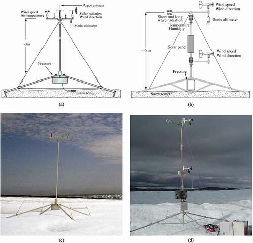
Table 3. Overview of available data in percentages per AWS for three different periods

		1993–2002	2003–2016
Period	1993–2016	Type I	Type II
S5	94	85	>99
S6	83	80	85
S9	/	47	>99
S10	/	/	>99

Figure 3. Overview of the available AWS data along the K-transect for the period from August 1993 to August 2016. For every year, all days of the year (DOY) with available data are plotted as colored vertical bars for every AWS. The grey part in 2016 at S10 indicates that for this period PROMICE AWS data are used. Purple horizontal bars indicate what type of AWS was used: 1 AWS Type I, 2 AWS Type II, and during periods (A) and (B) only a surface height ranger was present at locations S5 and S6, respectively

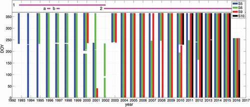
Figure 4. Mean JJA values for (A) air temperature, (B) shortwave incoming radiation, (C) albedo, and (D) longwave incoming radiation for AWS S5, S6, S9, and S10. Subplot (A) includes air-temperature data from the DMI meteorological station at Kangerlussuaq airport

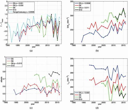
Figure 5. (A) NAO index anomalies relative to the 1981–2010 baseline and averaged each year for summer months (JJA). (B) Normalized values of the mean November–February precipitation and temperature at Kangerlussuaq, the NAO index, and the temperature at S9

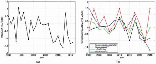
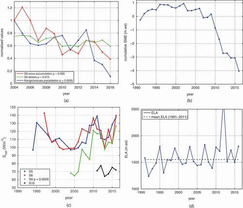
Figure 6. (A) Normalized yearly snow accumulation at S9, winter precipitation at Kangerlussuaq airport, and mean JJA albedo at S9; (B) cumulative SMB (m w.e.) at S9; (C) JJA mean net SW radiation at S5, S6, S9, and S10; (D) Equilibrium Line Latitude (ELA), defined as the altitude where SMB = 0, as estimated from inter/extrapolation of annual SMB profiles (van de Wal et al. 2012)

van de Wal, R. S. W., W. Boot, C. J. P. P. Smeets, H. Snellen, M. R. van den Broeke, and J. Oerlemans. 2012. Twenty-one years of mass balance observations along the K-transect, West. Western Greenland. Earth System Science Data 4:31–35. https://doi.org/https://doi.org/10.5194/essd-4-31-2012.

 Web of Science ®Google Scholar