Observed sediment and solute transport from the Kangerlussuaq sector of the Greenland Ice Sheet (2006–2016)

Figures & data

Figure 1. (A) GrIS catchment after Lindbäck et al. (2015); (B) proglacial area; and (C) Watson River and the fjord Kangerlussuaq

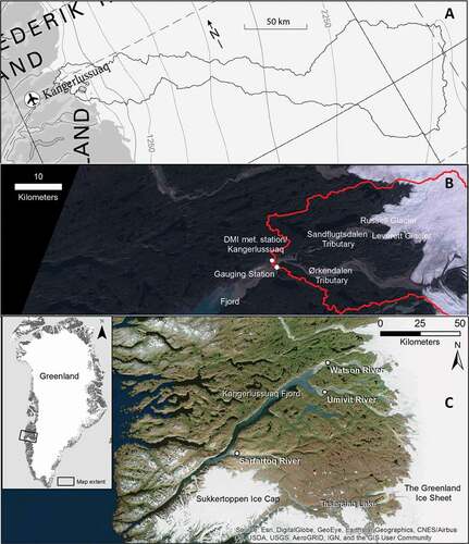
Figure 2. Gaging station at bridge crossing during low runoff (April 19, 2016) and high runoff (July 25, 2016)

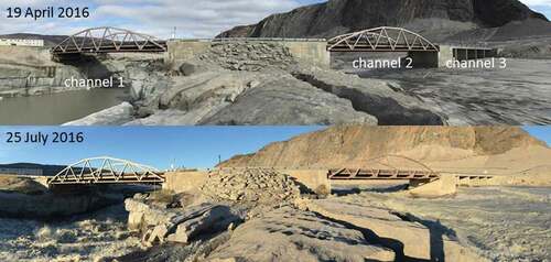
Figure 3. Seasonal variations of discharge. Years 2007, 2010, 2012, and 2013 are shown specifically. Peaks in August–September are jökulhlaup events (e.g., 2007)

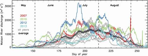
Table 1. Modeled transport characteristics of sediment and solutes in Watson River

	2006	2007	2008	2009	2010	2011	2012	2013	2014	2015	2016	Average	SD
Discharge (km^3 a^−1)	5.4	7.5	5.5	4.9	11.2	7.8	10.7	4.3	6.8	3.8	8.1	6.9	2.5
Sediment
Number of samples	7	24	50	67	184	48	77	29		1	16
Mean concentration (mg l^−1)	1930	3011	1917	2400	2358	2350	2638	1369		1568	1369	2089	552
Maximum concentration (mg l^−1)	8255	5427	6257	5943	5117	4095	5113	4264		1568	3163	4920	1817
Method 1 (× 10^6 t a^−1)			9.3	10.6	26.4	21.0	28.4	10.2				17.6	8.7
Method 2 (× 10^6 t a^−1)	13.1	19.1	13.1	12.7	24.6	20.5	30.5	7.9	13.9	7.8	18.6	16.5	6.9
Method 3 (× 10^6 t a^−1)	13.1	19.4	13.2	11.4	29.6	20.2	29.3	10.2	16.9	8.7	20.9	17.5	7.2
Method deviation (%)	0	2	22	10	10	1	4	16	10	6	6	4
Specific transport (t km^−2 a^−1)	1040	1537	1038	909	2353	1606	2325	810	1345	693	1658	1392	573
Solutes
Total solute export(× 10^3 t a^−1)	66.5	84.7	70.7	60.8	138.2	95.6	132.0	53.9	83.1	46.6	99.8	84.7	29.9
Specific transport(t km^−2 a^−1)	5.3	6.7	5.6	4.8	11.0	7.6	10.5	4.3	6.6	3.7	7.9	6.7	2.4

Figure 4. (A) Sampled sediment concentration plotted against river discharge. The red line represents the best exponential fit; dashed lines give the root mean square difference. (B) Sediment concentration versus OBS sensor readings. The red line is the fit following Hasholt et al. (2013). (C) Sediment concentration versus Solitech sensor readings. The red line is the fit following Hasholt et al. (2013)

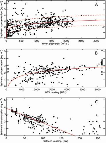
Figure 5. Annual totals and uncertainty of sediment transport through the Watson River

Table 2. Characteristics of sediments and solutes in Watson River, 2006–2016. Solute concentrations are shown as annual-mean ion concentrations based on the discharge-weighted method

	2006	2007	2008	2009	2010	2011	2012	2013	2014	2015	2016	Average	Stdev
Average loss on ignition (%)	1.9	1.5	1.2	1.2	1.2	0.4	0.2	2.7		1.0	1.4	1.27	0.71
Maximum (%)	3.2	1.9	4.7	6.0	3.5	2.2	0.69	6.9			3.0	3.57	1.99
Minimum (%)	1.1	1.2	0.4	0.4	0.4	0.02	0.1	0.7			0.4	0.52	0.41
Average 0.7–0.45 μm fraction (mg l^−1)	7.7	13.9	9.5	0	44.3							15.1	15.3
Maximum (mg l^−1)	11.7	15.5	44.8	0	68.9							28.2	25.1
Minimum (mg l^−1)	1.8	12.4	0	0	21.2							7.1	8.4
Average grain size (µm)				8.9	154.8
Max. (μm)				13.9	227.9
Min. (μm)				5.4	118.3
<20 μm fraction (%)				71	7.5
Na^+ mg l^−1		0.75	0.84	0.81				0.76				0.79	0.002
K^+ mg l^−1		0.79	0.92	0.89				1.05				0.91	0.006
Ca^2+ mg l^−1		1.32	1.68	1.79				2.14				1.73	0.19
Mg^2+ mg l^−1		0.20	0.20	0.25				0.33				0.25	0.003
Cl^− mg l^−1		1.07	1.02					0.44				0.84	0.15
NO3^− mg l^−1		0.15	0.16									0.15	0.0002
SO4^2- mg l^−1		1.54	1.77	1.55								1.62	0.006
HCO3^− mg l^−1		4.32	5.65									4.98	0.29
Si mg l^−1		1.07	0.65	1.17								0.96	0.12
Fe mg l^−1		0.08		0.03				0.05				0.05	0.01

Table 3. Sediment annual mass balance estimates for the Watson River catchment, 2009–2012

		Leverett Glacier		Russell Glacier	Ørkendalen Tributary	Total GrIS Input	Watson River Export			Proglacial Deposition
Year	Specific Sediment Transport	Sediment Transport^a	Uncertainty^a	Sediment Transport	Sediment Transport	Sediment Transport	Sediment Transport	Uncertainty	Specific Sediment Transport	Sediment Loss
	(t km^−2 a^−a)	(x 10^6 t a^−a)		(x 10^6 t a^−a)	(x 10^6 t a^−a)	(x 10^6 t a^−a)	(x 10^6 t a^−a)		(t km^−2 a^−a)	(× 10^6 t a^−a)
2009	15,000	9	±39%	0.53	27	36.5	11.4	±25%	910	25.1
2010	10,100	6	±39%	0.35	18.2	24.6	29.6	±25%	2,350	−5.0
2011	11,700	7	±39%	0.41	21	28.4	20.2	±25%	1,610	8.2
2012	8,500	5	±39%	0.30	15.3	20.7	29.3	±25%	2,330	−8.6
Average	11,300	6.8				27.6	22.6		1,800	4.9
SD	2,800	1.7				6.7	8.7		690	15.3

^aFrom Cowton et al. (2012) and Hawkings et al. (2015)

Table 4. Past, present, and future estimates of ion fluxes (× 10³ t yr⁻¹) from the GrIS based on upscaling from the Watson River catchment. The mean GrIS runoff fluxes are derived from Lenaerts et al. (2015). Two climate scenarios are used for estimating future ion fluxes. The RCP2.6 scenario has a modest increase in atmospheric temperature over Greenland until 2100 (c. 2 K), followed by a slow decrease. The RCP8.5/4xCO₂ scenario has a strong increase in atmospheric temperature over Greenland (c. 5 K in 2100)

	Runoff	Na^+	K^+	Ca^2+	Mg^2+	Cl^−	NO3^−	SO4^2-	HCO3^−	Si	Fe
	(km^3 yr^−1)	(× 10^3 t yr^.1)
1960–1989	394	311	358	677	96	337	60	640	1,959	380	20
2006–2016	652	515	592	1,120	159	557	98	1,059	3,241	629	33
2090–2099 (RCP2.6)	800	631	727	1,374	195	684	121	1,299	3,975	772	41
2090–2099 (RCP8.5/4xCO2)	1,581	1,247	1,435	2,715	384	1,350	239	2,565	7,853	1,525	81

Lindbäck, K., R. Pettersson, A. L. Hubbard, S. H. Doyle, D. van As, A. B. Mikkelsen, and A. A. Fitzpatrick. 2015. Subglacial water drainage, storage, and piracy beneath the Greenland Ice Sheet. Geophysical Research Letters 42:7606–14.

 Web of Science ®Google Scholar

Hasholt, B., A. B. Mikkelsen, M. H. Nielsen, and M. A. D. Larsen. 2013. Observations of runoff and sediment and dissolved loads from the Greenland Ice Sheet at Kangerlussuaq, West Greenland, 2007 to 2010. Zeitschrift Für Geomorphologie 57 (Suppl. 2):3–27.

 Google Scholar

Cowton, T., P. Nienow, I. Bartholemew, A. Sole, and D. Mair. 2012. Rapid erosion beneath the Greenland Ice Sheet. Geology 40:343–46.

 Web of Science ®Google Scholar

Hawkings, J. R., J. L. Wadham, M. Tranter, E. Lawson, A. Sole, T. Cowton, A. J. Tedstone, I. Bartholomew, P. Nienow, D. Chandler, et al. 2015. The effect of warming climate on nutrient and solute export from the Greenland Ice Sheet. Geochemical Perspectives Letters 1:94–104.

 Web of Science ®Google Scholar

Lenaerts, J. T. M., D. Le Bars, L. van Kampenhout, M. Vizcaíno, E. M. Enderlin, and M. R. van den Broeke. 2015. Representing Greenland Ice Sheet freshwater fluxes in climate models. Geophysical Research Letters 42:6373–81.

 Web of Science ®Google Scholar