Figures & data
Table 1. Geographic, climatic, and plant sociologic characteristics of the study sites along the elevational gradient in the European Alps from low to high. All vegetation-period specific values are site specific. Data shown were calculated from on-site weather-station data. Long-term data for Esterberg are not available.
Table 2. Experimental setup. Number of monoliths translocated from origin (rows) to recipient sites (columns).
Figure 1. Scheme of experimental setup. Each colored plant represents nine plant-soil monoliths, either translocated as control at the respective origin or to a specific recipient site. Colors of plants represent the investigated temperature gradient, from cold (blue) to warm (red). The grey scale of the mountain represents ecological zones spanned along this elevational gradient, ranging from colline (low elevation) to montane to alpine (high elevation).
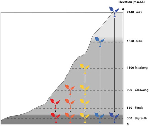
Figure 2. (a) Aboveground biomass and (b) Species richness change of plant communities in response to changes in elevation, growing degree days and precipitation resulting from downslope translocation. Significant influence of altered environmental conditions are shown as a black line with grey-shaded 95% confidence intervals. Significance of model factors indicated by asterisk (*** p < .001; ** p < .01; * p < .05; n.s non-significant) and overall model R2 are displayed in the lower right corner of the respective panel. Mean and standard error are displayed in all graphs. For the control monoliths mean and standard error was calculated for all controls grouped. Color code of legend is valid for all panels.
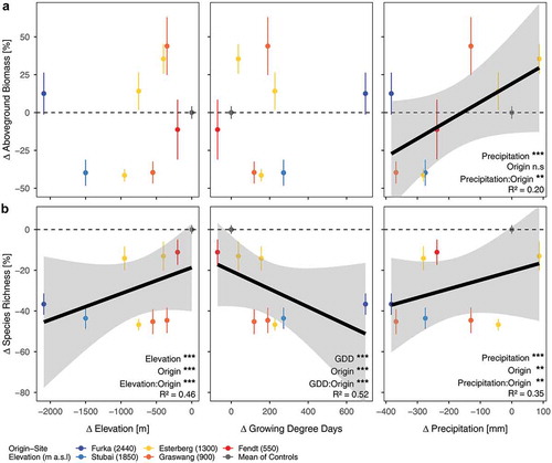
Figure 3. (a) Aboveground biomass and (b) species richness change in plant communities (monoliths) after one year of passive warming by translocation. Relative change for plant communities of all origins translocated downslope to the respective recipient site (m a.s.l. given) grouped together. Replicates at each recipient site given at the bottom of each panel. Mean and standard error are displayed in all graphs. Letters indicate significant differences between recipient sites as results of TukeyHSD post hoc tests conducted after ANOVA p < .001.
Figure 4. Green cover of translocated plant communities to the lowest elevation site (Bayreuth) showing different speed in greening up and different reaction to low soil-moisture availability. Green cover modeled as GAM shown as solid green line with 95 percent confidence intervals (dashed lines). Blue lines indicate soil moisture for the specific site of origin at the lowest elevation site (350 m a.s.l.). Red line shows harvest date at the recipient site (Bayreuth).
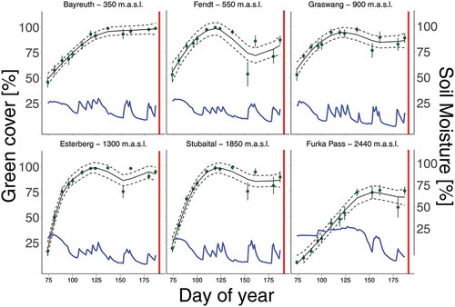
Figure 5. Changes in aboveground biomass and species richness showing relationship of relative change compared to the specific controls of (a) aboveground biomass versus light transmission, (b) aboveground biomass versus species richness, (c) light transmission versus species richness, and (d) proportion of graminoids versus species richness. Black lines with grey-shaded 95 percent confidence intervals are the overall model estimate; R2 and p values are given if significant. Colored lines represent site-of-origin model estimates.
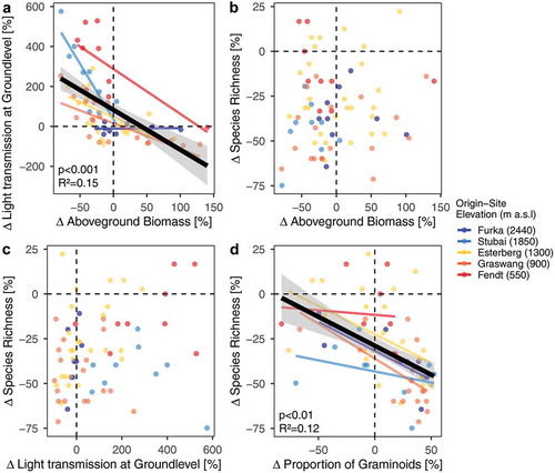
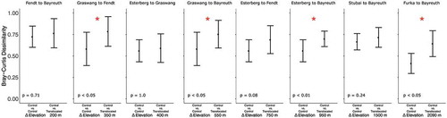
Figure 6. Dissimilarity in community composition among plant communities translocated along an elevational gradient from 2,440 m a.s.l. to 350 m a.s.l. Bray-Curtis dissimilarity values among indicated plant community (monolith) groupings for each monolith origin-translocated pairing. Panels are sorted according to elevational distance traveled by plant communities via translocation. Plotted values are means of all possible pairwise values in the indicated grouping with standard deviation error bars. PERMANOVA was used to test “within control dissimilarities” versus “between control/translocated” dissimilarities. Red asterisks indicate the significance between the translocated and control dissimilarities at p < .05 after adjusting for the multiple comparisons made within each origin group, additional p values are given in the lower left corner of each panel.