Figures & data
Figure 1. Study-area location and position of the sampled trees at the two study sites: GL (along the glacier stream) and SL (toward the valley slope). The photo refers to the tree marked by an asterisk, and was taken toward the southeast direction The position of the two latero-frontal moraines of the Forni Glacier in 1914 and in 1926 is also depicted. Coordinates refer to the UTM zone 32 N.
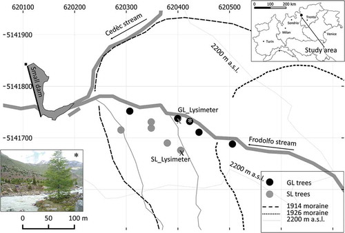
Table 1. Statistics calculated between standard chronologies (RWI = ring-width index), δ13C, and δ18O chronologies at the SL and SL sites, during the period 1980–2010 (n = 31): Glk = Gleichläufigkeit (Glk), correlation coefficient (CC), and t value. Significance level: * = p < .05; ** = p < .01; *** = p < .001.
Figure 2. The two ring-width standard chronologies constructed at the GL and SL study sites and the corresponding number of trees available in each year.
Figure 3. (a) The two δ13C chronologies and the two δ18O chronologies; (b) at the GL and SL sites together with the respective regression lines with equations; in (c) and (d) the δ13C and the δ18O yearly differences GL–SL are depicted together with the regression lines with equations and standard errors of the regression parameters.
Figure 4. Correlation coefficients calculated during the period 1980–2010 between monthly variables of temperature and precipitation from June of the year prior to growth (−1) to current September, and the following chronologies: (a) ring-width index, (b) δ13C, and (c) δ18O. Additionally, the same analysis is performed (d) between seasonal temperature variables and tree-ring δ18O and (e) between tree-ring δ18O and monthly and seasonal precipitation δ18O. The variable aggregation in (d) and (e) refers to mean temperature values calculated from the two preceding seasonalized variables along the x-axis. Statistically significant values: *p < .05; **p < .01; ***p < .001. In (a), (b), (c), and (e) values are related to the SL site as in (Leonelli et al. Citation2017).
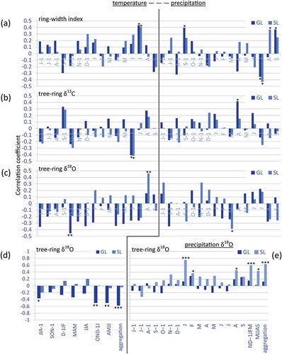
Figure 5. Linear regression between the cellulose δ18O at the GL and SL sites (black dots and gray points, respectively) and (a) the mean temperature of the months from October prior to growth (−1) to the current January, (b) the months from April to July, and (c) the aggregation of these two variables. The linear regression equation is reported for all regressions, as well as the corresponding equations, standard errors of the regression parameters, and determination coefficients. Statistically significant regressions: *p < .01; ***p < .001.
Table 2. Values of δ18O for the years and summer months (July to September) of 2013, 2014, and 2016 at the Forni site: precipitation δ18O (estimated values from the Pontresina series, equation 1; GL stream δ18O (measured values). The table also reports three columns of some noteworthy differences in δ18O, and four rows of the JAS means and general means during the three years of observations, together with the respective standard deviations (σ).
Figure 6. Climate data and water δ18O values for 2016: temperature and precipitation monthly values (CRU dataset ver. 4.0, Harris et al. Citation2014), δ18O of the lysimeters at SL and GL sites, δ18O measured in the GL stream, and δ18O of the Forni site derived from the Pontresina station, applying equation 1: the thin blue lines depict the associated error (± 0.72‰).
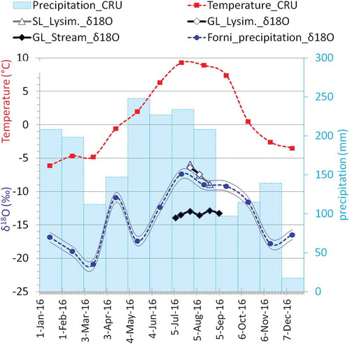
Figure 7. (a) Soil-water δ18O at the SL site is depicted with a grey line together with ± 1 standard deviation lines (SDEV), and the expected soil water δ18O at the GL site during the 1980–2010 period is depicted with a dashed line: in both cases (equations 2 and 4, respectively) the soil surface fractionation factor was set to zero, f = 0. In the bottom, the blue histogram bars depict the annual GMWI δ18O calculated with equation 5 and the green line depicts the values of ONDJ–AMJJ mean temperatures expressed as z-scores (−1 refers to months prior to growth). (b) Regression of the GMWI δ18O as function of ONDJ–AMJJ mean temperatures is expressed in °C; the regression line also reports the equations as well as the standard errors of the regression parameters and the determination coefficient.
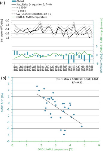
Figure 8. Cumulative front variations of the Forni Glacier during the period 1980–2010 (WGMS Citation2017), smoothed with a fifteen-year Gaussian curve.