Environmental changes of the last 1000 years on Prince of Wales Island, Nunavut, Canada

Figures & data

Figure 1. Sites with paleoclimate reconstructions of the past 1,000–2,000 years used in this study. Lake sediment records are denoted by a circle and color-coded by proxy type. The new record from this study is indicated in red (SW08).

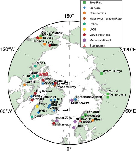
Table 1. Pollen and spore taxa identified in core SW08. The local and regional taxa were used in numerical analyses. Taxa denoted with an asterisk (*) were part of the modern training set but were not found in the core.

Local and Regional
Betula	Saxifraga oppositifolia
Alnus	Saxifragaceae undiff
Salix	Polygonaceae undiff
Ericaceae	Ranunculaceae undiff
Artemisia	Thalictrum*
Caryophyllaceae	Rosaceae undiff
Chenopodiaceae	Potentilla*
Brassicaceae	Rubus chamaemorus
Asteraceae	Lycopodium annotinum*
Cyperaceae	L. clavatum*
Dryas	Huperzia selago*
Poaceae	Lycopodium undiff
Fabaceae*	Selaginella
Oxyria	Polypodiaceae*
Papaver	Equisetum
Pedicularis*	Sphagnum
Long Distance Picea undiff Abies Pinus Populus Carpinus/Ostrya Juglans Acer Juniperus Fraxinus Morus Celtis Corylus Ulmus Urtica

Table 2. ²¹⁰Pb results and ages based on constant-rate-of-supply (CRS) (Appleby and Oldfield 1978) model. The supported activity for all samples was 64.0 Bq/kg.

Top Depth (cm)	Bottom Depth (cm)	Midpoint Depth (cm)	Subsample weight (mg)	Unsupported Activity (Bq/kg)	Year CE	CRS Error (years)
		0.0		134.78	2017	0.00
0.0	0.5	0.25	763.80	78.22	2015	0.23
0.5	1.0	0.75	786.60	132.24	2011	0.72
1.0	1.5	1.25	750.70	137.30	2004	1.25
1.5	2.0	1.75	719.10	152.96	1993	2.12
3.0	3.5	3.25	386.40	18.89	1962	7.23
6.0	6.5	6.25	537.50	12.73	1920	17.90
8.0	8.5	8.25	841.90	0.00	1880	19.11
8.5	9.0	8.75	837.20	22.39	N/A

Table 3. Radiocarbon ages and hardwater-corrected dates. *: Indicates dates rejected and not used in developing the chronology. All dates are based on aquatic mosses extracted from the sediment. Samples were calibrated using OxCal v4.2.4 (Bronk Ramsey 2009) and the IntCal13 calibration curve (Reimer et al. 2013).

Lab ID	Depth (cm)	^14C yr BP	Error (±)	2σ cal BP range	Median cal BP	Hard watercorrected median cal BP
*UOC‐5309	12–13	1961	29	1,830–1,989	1,909.5	N/A
UOC‐5310	15–16	1449	26	1,300–1,385	1,342.5	486.5
UOC‐5311	19–20	1647	24	1,441–1,613	1,527	671
UOC‐5312	25–26	1812	34	1,623–1,825	1,724	868
*UOC‐5313	37–38	1756	24	1,600–1,727	1,663.5	N/A
*UOC‐5314	45–46	1710	24	1,556–1,696	1,626	N/A

Figure 2. Age-depth curve for core SW08. Triangles are ²¹⁰Pb ages; Circles are the ¹⁴C median calibrated dates with 2σ age range; red circles are ¹⁴C dates rejected from age-depth model; Squares are hardwater-corrected ¹⁴C dates (see text for details). Solid line represents the corrected age-depth model; dashed line is the age-depth model without hardwater correction.

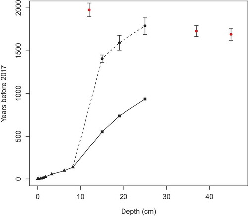
Figure 3. Local and regional pollen in core SW08. The second line in the curves of the rarer taxa is a 5x exaggeration. Sums were calculated based on entire pollen assemblage (local, regional, and long-distance), although the numbers in the final column include all pollen and spores counted.

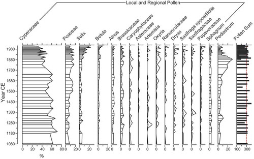
Figure 4. Long-distance, local, and regional pollen percentages, pollen concentrations, accumulation rates, and mean July temperature (°C) reconstruction for core SW08. Sums were calculated based on entire pollen assemblage (local, regional and long-distance). On the temperature reconstruction, grey lines are the standard deviation of the three best analogs and the red line is a loess curve (span = 0.25) fitted to the reconstruction.

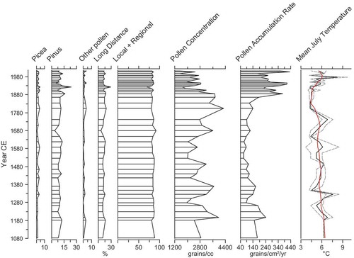
Figure 5. Principal Component Analysis (PCA) for SW08 pollen percentages. Only taxa used in the July temperature reconstruction were included in the PCA (Table 1). Panel (a) shows the loadings and (b) shows the scores coloured by year CE and grouped by climatic periods identified in the literature.

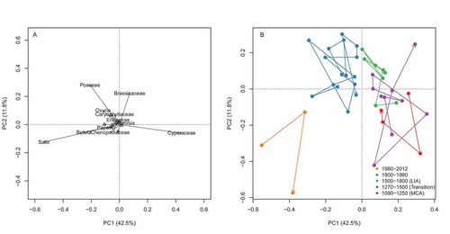
Figure 6. Pollen-based temperature reconstructions in the Central and Western Arctic. The horizontal line is the mean for each record based on a reference period from 1000–2000 CE. Note: the reconstructions for SL06, JR01, and MB01 differ from the original publications because they were redone using the new modern database from Gajewski (2015).

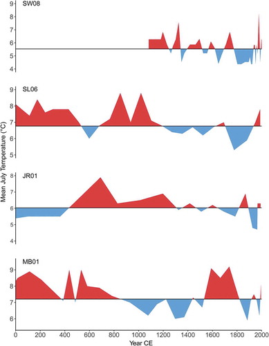
Figure 7. (A) Comparison of the average of all the records (n = 40) relative to their common period (1090–1960 CE; orange line) computed for this study and the average for all the records (standard deviation with respect to 980–1800 CE; blue line) from Kaufman et al. (2009). The solid gray line shows the number of records used to compute the average for this study over time (orange line). (B) Average for this study with (orange line) and without (blue line) additional records from the Canadian Arctic Archipelago. (C) Average for this study (orange line) and the PaiCo reconstruction (blue) from McKay and Kaufman (2014). Note: McKay and Kaufman (2014) is a reconstruction of annual temperature anomalies, whereas the averages from this study and Kaufman et al. (2009) are standardized values (z-scores).

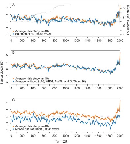
Figure 8. Principal Component Analysis (PCA) of proxy climate records from the Arctic. (A) Records from 1090–1960 CE (PCA₁) showing the loadings colored by proxy type. (B) Scores grouped by clusters established using Ward’s method. (C) Records from 10–1960 CE (PCA₂) showing loadings colored by proxy type (same legend as in panel A). (D) Scores grouped by clusters established using Ward’s method. Note the different axis scales.

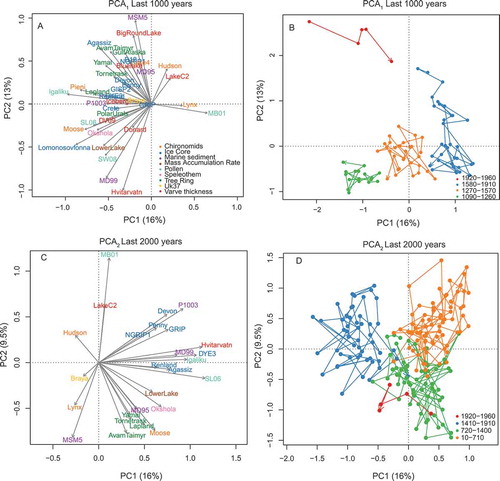
Figure 9. (A) Maps of the loadings from PCA₁ and associated scores over time for component 1 and (B) component 2. (C) Maps of loadings from PCA₂ and associated scores over time for component 1 and (D) component 2.

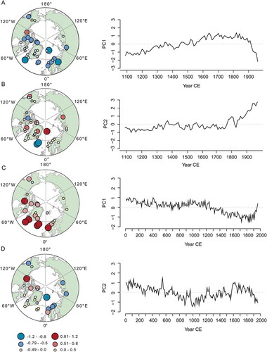
Table A1. List of reconstructions included in the synthesis study. Sites in bold are included in both PCA₁ (1090–1960 CE) and PCA₂ (10–1960 CE).

Site	Region	Lat	Long	Archive	Proxy	Reference
Arc_1_Bluelake	Alaska	68.1	−150.5	Lake sediment	Varve thickness	Bird et al. (2009)
Arc_7_GulfAlaska	Alaska	61.0	−146.6	Tree Ring	Ring width	Wiles et al. (2014)
Arc_41_Hudson	Alaska	61.9	−145.7	Lake sediment	Chironomids	Clegg et al. (2011)
Arc_42_lynx	Alaska	66.1	−145.4	Lake sediment	Chironomids	Clegg et al. (2011)
Arc_40_Moose	Alaska	61.3	−143.6	Lake sediment	Chironomids	Clegg et al. (2010)
Arc_23_Iceberg	Alaska	60.8	−143.0	Lake sediment	Varve thickness	Loso et al. (2006)
MB01	Victoria Island, NWT	69.8	−112.1	Lake sediment	Pollen	Peros and Gajewski (2009)
SW08	Prince of Wales Isl, NU	72.3	−97.27	Lake sediment	Pollen	Tamo and Gajewski, this volume
SL06	Boothia Peninsula, NU	68.6	−91.9	Lake sediment	Pollen	Peros and Gajewski (2009)
DV09	Devon Island, NU	75.6	−89.3	Lake sediment	Varve thickness	Courtney Mustaphi and Gajewski (2013)
Arc_54_Lake4	Southampton Isl, NU	65.1	−83.8	Lake sediment	Chironomids	Rolland et al. (2009)
Arc_44_Devon	Devon Island, NU	75.3	−82.5	Ice core	δ^18O	Fisher et al. (1983)
Arc_20_LakeC2	Ellesmere Island, NU	82.1	−77.2	Lake sediment	Varve thickness	Lamoureux and Bradley (1996)
Agassiz Ice Cap	Ellesmere Island, NU	81.0	−75	Ice core	δ^18O	Lecavalier et al. (2017)
Arc_4_Lower Lake	Ellesmere Island, NU	81.4	−69.5	Lake sediment	Mass accumulation rate	Cook et al. (2009)
Arc_30_BigRoundLake	Baffin island, NU	69.9	−68.8	Lake sediment	Varve thickness	Thomas and Briner (2009)
Arc_53_Penny	Baffin Island, NU	67.3	−66.8	Ice core	δ^18O	Fisher et al. (1998)
Arc_25_Donard	Baffin Island, NU	66.7	−61.4	Lake sediment	Varve thickness	Moore et al. (2001)
Arc_43_Braya	Greenland	67.0	−50.7	Lake sediment	U^K’37	D’Andrea et al. (2011)
Arc_52_Igaliku	Greenland	61.0	−45.4	Lake sediment	Pollen accumulation	Massa et al. (2012)
Arc_35_DYE3	Greenland	65.2	−43.8	Ice core	δ^18O	Vinther et al. (2010)
Arc_32_NGRIP1	Greenland	75.1	−42.3	Ice core	δ^18O	Vinther et al. (2006)
Arc_11_GISP2	Greenland	72.1	−38.1	Ice core	δ^18O	Grootes and Stuiver (1997)
Arc_36_GRIP	Greenland	72.6	−37.6	Ice core	δ^18O	Vinther et al. (2010)
Arc_34_Crete	Greenland	71.1	−37.3	Ice core	δ^18O	Vinther et al. (2010)
Arc_28_B18	Greenland	76.6	−36.4	Ice core	δ^18O	Schwager (2000)
Arc_59_Renland	Greenland	71.3	−26.7	Ice core	δ^18O	Vinther et al. (2008)
Arc_22_Hvitarvatn	Iceland	64.6	−19.8	Lake sediment	Varve thickness	Larsen et al. (2011)
Arc_57_MD99-2275	North Atlantic	66.6	−17.4	Marine sediment	U^K’37	Sicre et al. (2011)
Arc_55_P1003	North Atlantic	63.8	5.3	Marine sediment	δ^18O	Sejrup, Haflidason, and Andrews (2011)
Arc_58_MSm5/5–712	North Atlantic	78.9	6.8	Marine sediment	Planktic forams	Spielhagen et al. (2011)
Arc_38_MD95-2011	North Atlantic	67.0	7.6	Marine sediment	Diatoms	Berner et al. (2011)
Arc_49_Okshola Cave	Scandinavia	67	15	Speleothem	δ^18O	Linge et al. (2009)
Arc_17_Lomonosovfonna	North Atlantic	78.9	17.4	Ice core	δ^18O	Divine et al. (2011)
Arc_12_Tornetrask	Scandinavia	68.3	19.6	Tree Ring	Ring Width	Grudd (2008)
Arc_15_Lapland	Scandinavia	69.0	25.0	Tree Ring	Ring width	Helama et al. (2009)
Arc_51_Pieni	Scandinavia	64.3	30.1	Lake sediment	Chironomids	Luoto and Helama (2010)
Arc_10_PolarUrals	Central Russia	66.8	65.8	Tree Ring	Max. density	Esper, Cook, and Schweingruber (2002)
Arc_3_Yamal	Central Russia	67.5	70.0	Tree Ring	Ring width	Briffa et al. (2008)
Arc_2_AvamTaimyr	Central Russia	72.0	101.0	Tree Ring	Ring width	Briffa et al. (2008)

Appleby, P. G., and F. Oldfield. 1978. The calculation of lead-210 dates assuming a constant rate of supply of unsupported 210Pb to the sediment. Catena 5 (1):1–8. doi:10.1016/S0341-8162(78)80002-2.

 Google Scholar

Bronk Ramsey, C. 2009. Bayesian analysis of radiocarbon dates. Radiocarbon 51 (1):337–60. doi:10.1017/S0033822200033865.

 Web of Science ®Google Scholar

Reimer, P. J., E. Bard, A. Bayliss, J. W. Beck, P. G. Blackwell, C. B. Ramsey, C. E. Buck, H. Cheng, R. L. Edwards, M. Friedrich, et al. 2013. IntCal13 and Marine13 radiocarbon age calibration curves 0–50,000 years cal BP. Radiocarbon 55 (4):1869–87. doi:10.2458/azu_js_rc.55.16947.

 Web of Science ®Google Scholar

Gajewski, K. 2015. Quantitative reconstruction of Holocene temperatures across the Canadian Arctic and Greenland. Global and Planetary Change 128:14–23. doi:10.1016/j.gloplacha.2015.02.003.

 Web of Science ®Google Scholar

Kaufman, D. S., D. P. Schneider, N. P. McKay, C. M. Ammann, R. S. Bradley, K. R. Briffa, G. H. Miller, B. L. Otto-Bliesner, J. T. Overpeck, B. M. Vinther, et al. 2009. Recent warming reverses long-term Arctic cooling. Science 325 (5945):1236–39. doi:10.1126/science.1173983.

 PubMed Web of Science ®Google Scholar

McKay, N. P., and D. S. Kaufman. 2014. An extended Arctic proxy temperature database for the past 2,000 years. Scientific Data 1:140026. doi:10.1038/sdata.2014.26.

 Web of Science ®Google Scholar

Bird, B. W., M. B. Abbott, B. P. Finney, and B. Kutchko. 2009. A 2000 year varve-based climate record from the central Brooks Range, Alaska. Journal of Paleolimnology 41 (1):25–41. doi:10.1007/s10933-008-9262-y.

 Web of Science ®Google Scholar

Wiles, G. C., R. D. D’Arrigo, D. Barclay, R. S. Wilson, S. K. Jarvis, L. Vargo, and D. Frank. 2014. Surface air temperature variability reconstructed with tree rings for the Gulf of Alaska over the past 1200 years. The Holocene 24 (2):198–208. doi:10.1177/0959683613516815.

 Web of Science ®Google Scholar

Clegg, B. F., R. Kelly, G. H. Clarke, I. R. Walker, and F. S. Hu. 2011. Nonlinear response of summer temperature to Holocene insolation forcing in Alaska. Proceedings of the National Academy of Sciences 108 (48):19299–304. doi:10.1073/pnas.1110913108.

 Web of Science ®Google Scholar

Clegg, B. F., G. H. Clarke, M. L. Chipman, M. Chou, I. R. Walker, W. Tinner, and F. S. Hu. 2010. Six millennia of summer temperature variation based on midge analysis of lake sediments from Alaska. Quaternary Science Reviews 29 (23–24):3308–16. doi:10.1016/J.QUASCIREV.2010.08.001.

 Web of Science ®Google Scholar

Loso, M. G., R. S. Anderson, S. P. Anderson, and P. J. Reimer. 2006. A 1500-year record of temperature and glacial response inferred from varved Iceberg Lake, southcentral Alaska. Quaternary Research 66 (1):12–24. doi:10.1016/j.yqres.2005.11.007.

 Web of Science ®Google Scholar

Peros, M., and K. Gajewski. 2009. Pollen-based reconstructions of late Holocene climate from the central and western Canadian Arctic. Journal of Paleolimnology 41 (1):161–75. doi:10.1007/s10933-008-9256-9.

 Web of Science ®Google Scholar

Courtney Mustaphi, C. J., and K. Gajewski. 2013. Holocene sediments from a coastal lake on northern Devon Island, Nunavut, Canada. Canadian Journal of Earth Sciences 50 (5):564–75. doi:10.1139/cjes-2012-0143.

 Web of Science ®Google Scholar

Rolland, N., I. Larocque, P. Francus, R. Pienitz, and L. Laperrière. 2009. Evidence for a warmer period during the 12th and 13th centuries AD from chironomid assemblages in Southampton Island, Nunavut, Canada. Quaternary Research 72 (1):27–37. doi:10.1016/j.yqres.2009.03.001.

 Web of Science ®Google Scholar

Fisher, D. A., R. M. Koerner, W. S. B. Paterson, W. Dansgaard, N. Gundestrup, and N. Reeh. 1983. Effect of wind scouring on climatic records from ice-core oxygen-isotope profiles. Nature 301 (5897):205. doi:10.1038/301205a0.

 Web of Science ®Google Scholar

Lamoureux, S. F., and R. S. Bradley. 1996. A late Holocene varved sediment record of environmental change from northern Ellesmere Island, Canada. Journal of Paleolimnology 16 (2):239–55. doi:10.1007/BF00176939.

 Web of Science ®Google Scholar

Lecavalier, B. S., D. A. Fisher, G. A. Milne, B. M. Vinther, L. Tarasov, P. Huybrechts, D. Lacelle, B. Main, J. Zheng, J. Bourgeois, and A. S. Dyke. 2017. High Arctic Holocene temperature record from the Agassiz ice cap and Greenland ice sheet evolution. Proceedings of the National Academy of Sciences 114 (23):5952–57. doi:10.1073/pnas.1616287114.

 PubMed Web of Science ®Google Scholar

Cook, T. L., R. S. Bradley, J. S. Stoner, and P. Francus. 2009. Five thousand years of sediment transfer in a high arctic watershed recorded in annually laminated sediments from Lower Murray Lake, Ellesmere Island, Nunavut, Canada. Journal of Paleolimnology 41 (1):77. doi:10.1007/s10933-008-9252-0.

 Web of Science ®Google Scholar

Thomas, E. K., and J. P. Briner. 2009. Climate of the past millennium inferred from varved proglacial lake sediments on northeast Baffin Island, Arctic Canada. Journal of Paleolimnology 41 (1):209–24. doi:10.1007/s10933-008-9258-7.

 Web of Science ®Google Scholar

Fisher, D. A., R. M. Koerner, J. C. Bourgeois, G. Zielinski, C. Wake, C. U. Hammer, H. B. Clausen, N. Gundestrup, S.Johnsen, K. Goto-Azuma, et al. 1998. Penny ice cap cores, Baffin Island, Canada, and the Wisconsinan Foxe Dome connection: Two states of Hudson Bay ice cover. Science 279 (5351):692–95. doi:10.1126/science.279.5351.692.

 PubMed Web of Science ®Google Scholar

Moore, J. J., K. A. Hughen, G. H. Miller, and J. T. Overpeck. 2001. Little Ice Age recorded in summer temperature reconstruction from vared sediments of Donard Lake, Baffin Island, Canada. Journal of Paleolimnology 25 (4):503–17. doi:10.1023/A:1011181301514.

 Web of Science ®Google Scholar

D’Andrea, W. J., Y. Huang, S. C. Fritz, and N. J. Anderson. 2011. Abrupt Holocene climate change as an important factor for human migration in West Greenland. Proceedings of the National Academy of Sciences 108 (24):9765–69. doi:10.1073/pnas.1101708108.

 Web of Science ®Google Scholar

Massa, C., B. B. Perren, E. Gauthier, V. Bichet, C. Petit, and H. Richard. 2012. A multiproxy evaluation of Holocene environmental change from Lake Igaliku, South Greenland. Journal of Paleolimnology 48 (1):241–58. doi:10.1007/s10933-012-9594-5.

 Web of Science ®Google Scholar

Vinther, B. M., P. D. Jones, K. R. Briffa, H. B. Clausen, K. K. Andersen, D. Dahl-Jensen, and S. J. Johnsen. 2010. Climatic signals in multiple highly resolved stable isotope records from Greenland. Quaternary Science Reviews 29 (3–4):522–38. doi:10.1016/j.quascirev.2009.11.002.

 Web of Science ®Google Scholar

Vinther, B. M., H. B. Clausen, S. J. Johnsen, S. O. Rasmussen, K. K. Andersen, S. L. Buchardt, D. Dahl‐Jensen, I. K. Seierstad, M.‐L. Siggaard‐Andersen, J. P. Steffensen, et al. 2006. A synchronized dating of three Greenland ice cores throughout the Holocene. Journal of Geophysical Research: Atmospheres 111:D13. doi:10.1029/2005JD006921.

 Web of Science ®Google Scholar

Grootes, P. M., and M. Stuiver. 1997. Oxygen 18/16 variability in Greenland snow and ice with 10−3‐ to 105‐year time resolution. Journal of Geophysical Research: Oceans 102 (C12):26455–70. doi:10.1029/97JC00880.

 Web of Science ®Google Scholar

Schwager, M. 2000. Ice core analysis on the spatial and temporal variability of temperature and precipitation during the late Holocene in North Greenland. Reports on Polar Research 362:1–136. doi:10.2312/BzP_0362_2000.

 Google Scholar

Vinther, B. M., H. B. Clausen, D. A. Fisher, R. M. Koerner, S. J. Johnsen, K. K. Andersen, D. Dahl‐Jensen, S. O. Rasmussen, J. P. Steffensen, and A. M. Svensson. 2008. Synchronizing ice cores from the Renland and Agassiz ice caps to the Greenland Ice Core Chronology. Journal of Geophysical Research: Atmospheres 113:D8. doi:10.1029/2007JD009143.

 Web of Science ®Google Scholar

Larsen, D. J., G. H. Miller, Á. Geirsdóttir, and T. Thordarson. 2011. A 3000-year varved record of glacier activity and climate change from the proglacial lake Hvítárvatn, Iceland. Quaternary Science Reviews 30 (19–20):2715–31. doi:10.1016/j.quascirev.2011.05.026.

 Web of Science ®Google Scholar

Sicre, M., I. R. Hall, J. Mignot, M. Khodri, U. Ezat, M. Truong, J. Eiríksson, and K. Knudsen. 2011. Sea surface temperature variability in the subpolar Atlantic over the last two millennia. Paleoceanography 26:4. doi:10.1029/2011PA002169.

 Google Scholar

Sejrup, H. P., H. Haflidason, and J. T. Andrews. 2011. A Holocene North Atlantic SST record and regional climate variability. Quaternary Science Reviews 30 (21–22):3181–95. doi:10.1016/J.QUASCIREV.2011.07.025.

 Web of Science ®Google Scholar

Spielhagen, R. F., K. Werner, S. A. Sørensen, K. Zamelczyk, E. Kandiano, G. Budeus, K. Husum, T. M. Marchitto, and M. Hald. 2011. Enhanced modern heat transfer to the Arctic by warm Atlantic water. Science 331 (6016):450–53. doi:10.1126/science.1197397.

 PubMed Web of Science ®Google Scholar

Berner, K. S., N. Koç, F. Godtliebsen, and D. Divine. 2011. Holocene climate variability of the Norwegian Atlantic Current during high and low solar insolation forcing. Paleoceanography and Paleoclimatology 26:2.

 Google Scholar

Linge, H., S.-E. Lauritzen, C. Andersson, J. K. Hansen, R. Ø. Skoglund, and H. S. Sundqvist. 2009. Stable isotope records for the last 10000 years from Okshola cave (Fauske, northern Norway) and regional comparisons. Climate of the Past 5 (4):667–82. doi:10.5194/cp-5-667-2009.

 Web of Science ®Google Scholar

Divine, D., E. Isaksson, T. Martma, H. A. J. Meijer, J. Moore, V. Pohjola, R. S. W. van den Wal, and F. Godtliebsen. 2011. Thousand years of winter surface air temperature variations in Svalbard and northern Norway reconstructed from ice-core data. Polar Research 30 (1):7379. doi:10.3402/polar.v30i0.7379.

 Web of Science ®Google Scholar

Grudd, H. 2008. Torneträsk tree-ring width and density AD 500–2004: A test of climatic sensitivity and a new 1500-year reconstruction of north Fennoscandian summers. Climate Dynamics 31 (7–8):843–57. doi:10.1007/s00382-007-0358-2.

 Web of Science ®Google Scholar

Helama, S., M. Timonen, J. Holopainen, M. G. Ogurtsov, K. Mielikäinen, M., Eronen, M. Lindholm, and J. Meriläinen. 2009. Summer temperature variations in Lapland during the Medieval Warm Period and the Little Ice Age relative to natural instability of thermohaline circulation on multi-decadal and multi-centennial scales. Journal of Quaternary Science 24 (5):450–56. doi:10.1002/jqs.1291.

 Web of Science ®Google Scholar

Luoto, T. P., and S. Helama. 2010. Palaeoclimatological and palaeolimnological records from fossil midges and tree-rings: The role of the North Atlantic Oscillation in eastern Finland through the Medieval Climate Anomaly and Little Ice Age. Quaternary Science Reviews 29 (17–18):2411–23. doi:10.1016/J.QUASCIREV.2010.06.015.

 Web of Science ®Google Scholar

Esper, J., E. R. Cook, and F. H. Schweingruber. 2002. Low-frequency signals in long tree-ring chronologies for reconstructing past temperature variability. Science 295 (5563):2250–53. doi:10.1126/science.1066208.

 PubMed Web of Science ®Google Scholar

Briffa, K. R., V. V. Shishov, T. M. Melvin, E. A. Vaganov, H. Grudd, R. M. Hantemirov, M. Eronen, and M. M. Naurzbaev. 2008. Trends in recent temperature and radial tree growth spanning 2000 years across northwest Eurasia. Philosophical Transactions of the Royal Society of London B: Biological Sciences 363 (1501):2269–82. doi:10.1098/rstb.2007.2199.

 Web of Science ®Google Scholar