Potential shifts in zooplankton community structure in response to changing ice regimes and hydrologic connectivity

Figures & data

Figure 1. (a) Sample locations and timing in the (b) Fish Creek Watershed in northern Alaska, USA, approximately midway between Utqiaģvik and Prudhoe Bay along the Beaufort Sea coast and entirely within the National Petroleum Reserve – Alaska (NPR-A).

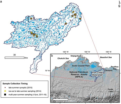
Table 1. Mean (± standard error) standardized water temperature (SWT), time from ice out, lake area, lake depth, and bedfast ice by connectivity index categories (1 = isolated, 4 = high hydrological connectivity).

Connectivity Index Category	1	2	3	4
n	5	17	10	8
SWT (°C)	8.0 (± 0.5)	9.5 (± 0.1)	9.6 (± 0.2)	10.7 (± 0.8)
Time from Ice Out (days)	31.6 (± 5.9)	50.4 (± 3.4)	40.0 (± 4.4)	42.6 (± 4.7)
Lake Area (km^2)	0.2 (± 0.04)	2.3 (± 0.4)	3.1 (± 0.7)	1.2 (± 0.7)
Depth (m)	2.2 (± 0.3)	4.3 (± 0.9)	4.9 (± 1.5)	2.8 (± 0.8)
Bedfast Ice Index	57.8 (± 13.0)	54.7 (± 7.2)	55.5 (± 8.7)	45.9 (± 10.9)

Table 2. Mean (± standard error) biomass (µg d.w. L⁻¹) of Daphnia spp. (n = 4 species), other cladocerans (n = 7 species), total cladocerans (n = 11 species), Heterocope sp., Diaptomidae (n = 6 species), other Calanoida (n = 3 species), total Calanoida (n = 10 species), total Cyclopoida (n = 5 species), total Rotifera (n = 54 species), and total phytoplankton biovolume (μm³ L⁻¹) for the connectivity index categories (1 = isolated, 4 = high hydrological connectivity); n represents the number of lakes in each connectivity index category.

Connectivity Index Category	1	2	3	4
n	5	17	10	8
Daphnid Biomass	41.5 (± 20.1)	33.5 (± 21.5)	9.5 (± 7.1)	18.3 (± 13.8)
Other Cladoceran Biomass	0.3 (± 0.1)	2.0 (± 1.2)	1.4 (± 0.7)	12.3 (± 8.5)
Total Cladoceran Biomass	41.8 (± 20.1)	35.6 (± 21.3)	11.0 (± 7.1)	30.5 (± 14.3)
Heterocope Biomass	1.44 (± 0.94)	0.94 (± 0.52)	0.42 (± 0.32)	0.15 (± 0.15)
Diaptomidae Biomass	12.61 (± 5.59)	19.03 (± 13.76)	2.56 (± 2.14)	1.68 (± 0.70)
Other Calanoida Biomass	0.04 (± 0.04)	0.01 (± 0.01)	0.52 (± 0.42)	0.14 (± 0.14)
Total Calanoida Biomass	14.1 (± 6.0)	19.98 (± 14.22)	3.5 (± 2.5)	2.0 (± 0.8)
Cyclopoida Biomass	**6.10 (± 2.41)	0.20 (± 0.11)	0.18 (± 0.09)	0.14 (± 0.13)
Rotifera Biomass	0.56 (± 0.27)	1.49 (± 0.33)	3.29 (± 1.05)	2.38 (± 0.72)
Phytoplankton Biovolume	1.34 x10^9 (± 4.81 × 10^8)	9.50 x 10^8 (± 1.19 × 10^8)	1.39 x 10^9 (± 1.74 × 10^8)	1.29 x 10^9 (± 1.85 × 10^8)

** denotes significant difference at p < 0.01.

Table 3. Mean (± standard error) weighted length (mm) for Daphnia spp. (n = 4 species), other cladocerans (n = 7 species), total cladocerans (n = 11 species), total Calanoida (n = 10 species), and total Cyclopoida (n = 5 species) for the connectivity index categories (1 = isolated, 4 = high hydrological connectivity); n represents the number of lakes in each connectivity index category. Mean weighted length based on relative abundance.

Connectivity Index Category	1	2	3	4
n	5	17	10	8
Daphnid Length	1.45 (± 0.25)	1.39 (± 0.27)	1.04 (± 0.25)	1.18 (± 0.34)
Other Cladoceran Length	0.37 (± 0.03)	0.34 (± 0.01)	0.43 (± 0.08)	0.42 (± 0.05)
Total Cladoceran Length	0.92 (± 0.20)	0.97 (± 0.23)	0.67 (± 0.16)	0.75 (± 0.15)
Calanoida Length	1.38 (± 0.19)	1.19 (± 0.12)	1.07 (± 0.14)	1.12 (± 0.15)
Cyclopoida Length	*1.64 (± 0.35)	0.87 (± 0.16)	0.80 (± 0.11)	0.99 (± 0.24)

* denotes significant difference at p < 0.05.

Table 4. Mean (± standard error) ratio of C-zooplankton to C-phytoplankton (Z:P) for the connectivity index category (1 = isolated, 4 = high hydrological connectivity).

	n	C-zooplankton:C-phytoplankton
Connectivity 1	5	0.19 (± 0.08)
Connectivity 2	17	0.10 (± 0.04)
Connectivity 3	10	0.03 (± 0.01)
Connectivity 4	6	0.07 (± 0.04)

Figure 2. Canonical Correlation Analysis (CCA) ordination diagrams for the zooplankton biomass CCA (n = 145) [(a) Daphnia middendorffiana; (b) Daphnia longiremis (light gray bubbles) and Daphnia pulex complex (dark gray bubbles); (c) Calanoida (d) Bosmina longirostris; (e) rotifers (light gray bubbles) and Cyclopoida (dark gray bubbles)]; and (f) samples coded by month. (a)–(e): each bubble represents biomass (zooplankton ordinations (a–e) µg d.w. L⁻¹) or biovolume (phytoplankton ordination (f) µm³ L⁻¹) for an individual sample, and bubble size corresponds to the magnitude of biomass in one sample according to the scale to the right of each ordination diagram. (f): each point represents a single sample, coded by month.

Table 5. Mean (± standard error) values for species richness, lake area, lake depth, and bedfast ice extent for each lake cluster identified from the complete linkage dendrogram.

	n	Mean Fish Species Observed	Lake Area (km^2)	Depth (m)	Bedfast Ice Extent
Cluster 1	10	2.2	1.5 (± 0.5)	3.1 (± 1.0)	53.6 (± 9.6)
Cluster 2	8	5.6	2.9 (± 0.8)	4.7 (± 1.2)	43.9 (± 5.0)
Cluster 3	4	4.8	2.7 (± 1.3)	6.1 (± 3.4)	50.6 (± 17.2)

Table 6. Mean (± standard error) biomass (µg d.w. L⁻¹) of B. longirostris, Calanoida, Cyclopoida, Daphnia spp., Rotifers, total zooplankton biomass and total phytoplankton biovolume (μm³ L⁻¹)for each lake cluster identified from the complete linkage dendrogram performed on fish community composition in lakes.

	n	B. longirostris	Calanoida	Cyclopoida	Daphnia spp.	Rotifers	Total Biomass	Total Biovolume
Cluster 1	10	1.1 (± 0.8)	5.5 (± 2.3)	2.3 (± 1.2)	36.4 (± 14.8)	2.0 (± 0.8)	54.5 (± 17.3)	1.0 x 10^9 (± 1.6 × 10^8)
Cluster 2	8	1.2 (± 0.5)	0.4 (± 0.3)	0.2 (± 0.1)	2.6 (± 1.8)	2.4 (± 0.6)	7.4 (± 2.9)	1.2 x 10^9 (± 2.3 × 10^8)
Cluster 3	4	1.5 (± 0.8)	4.8 (± 4.7)	3.1 (± 2.6)	13.7 (± 11.5)	3.0 (± 1.9)	34.1 (± 26.1)	1.1 x 10^9 (± 2.4 × 10^8)

Figure 3. Complete linkage dendrogram resulting from fish catch per unit effort (CPUE) data across 22 lakes. Clusters 1 through 3 represent ten, eight, and four lakes, respectively.

Figure 4. 2014 seasonal mean: (a) standardized water temperature, (b) zooplankton biomass, and (c) phytoplankton biovolume. Sampling events 1–4 correspond to mid-June, late June, mid-July, and mid-August, respectively. Data were analyzed according to connectivity index (connectivity 1, n = 16; connectivity 2, n = 16; connectivity 3, n = 20; connectivity 4, n = 12).

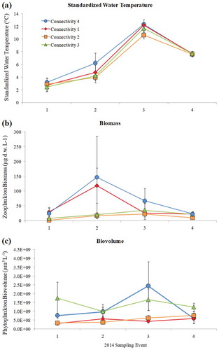
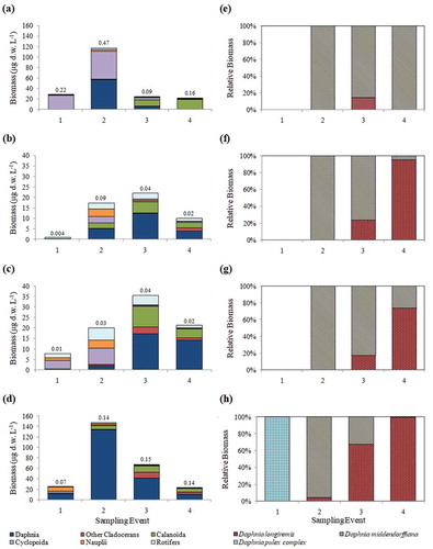
Figure 5. Mean zooplankton biomass and mean relative biomass of Daphnia species for 2014 seasonal sampling. Sampling events 1–4 correspond to mid-June, late June, mid-July, and mid-August, respectively. Data are organized by connectivity index with (a) connectivity 1, total biomass, (b) connectivity 2, total biomass, (c) connectivity 3, total biomass, (d) connectivity 4, total biomass, (e) connectivity 1, relative daphnid biomass, (f) connectivity 2, relative daphnid biomass, (g) connectivity 3, relative daphnid biomass, and (h) connectivity 4, relative daphnid biomass. Connectivity 1, n = 4 lakes; connectivity 2, n = 4 lakes; connectivity 3, n = 5 lakes; connectivity 4, n = 3 lakes). Mean Z:P ratio is given above bars in (a)–(d).