Combined effects of early snowmelt and climate warming on mountain lake temperatures and fish energetics

Figures & data

Figure 1. Raw Wilderness Area (RWA) of northern Colorado, United States, with location of the lakes in blue (R2 = Rawah #2, R3 = Rawah #3, R4 = Rawah #4) and approximate elevation topography (m.a.s.l.). The locations of the weather station (X), SNOTEL site (triangle), and Michigan River stream gauge (cross) are also shown

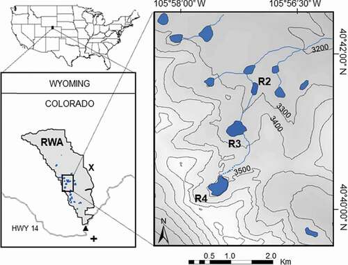
Figure 2. Daily snowpack depth (SWE) and lake surface temperatures and inflow temperature for Rawah #2 and Rawah #3 in 2016, as well as outflow temperature for Rawah #2. Date of ice-out in each lake is indicated. Polynomial functions fit to the inflows are shown as dotted lines

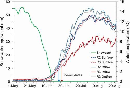
Figure 3. (a) Day of year when snowpack reached zero (snowmelt date; solid line) and yearly maximum snowpack depth (SWE; dashed line). (b) Frequency histogram of snowmelt dates. All snow data are from the Joe Wright SNOTEL station in north central Colorado, United States

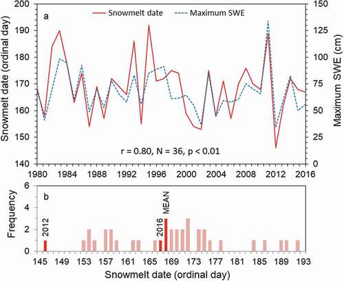
Figure 4. Streamflow from the Michigan River stream gauge for 2012 and 2016 (solid lines). Fitted exponential decay functions are shown for the duration of the open-water period each year (dotted lines)

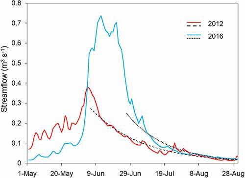
Table 1. Values of coefficients used to simulate lake inflow temperature and volume. $Temp=a{t}^2+bt+c$$R_0{e}^{-Kt}$

				Lake
Inflow parameter	Snowmelt scenario	Model coefficient	Air warming scenario	Rawah #2	Rawah #3
Volume	Nominal	R0		2.7	2.2
		K		−0.072	−0.072
	Early	R0		2.7	2.2
		K		−0.057	−0.057
Temperature	Nominal	a	Nominal		−0.0022
			+2°C		−0.0022
			+5°C		−0.0022
		b	Nominal		0.3541
			+2°C		0.3541
			+5°C		0.3541
		c	Nominal		−6.1194
			+2°C		−4.1194
			+5°C		−1.1194
	Early	a	Nominal		−0.0014
			+2°C		−0.0014
			+5°C		−0.0014
		b	Nominal		0.21
			+2°C		0.21
			+5°C		0.21
		c	Nominal		0.5
			+2°C		1.38
			+5°C		2.7

Note. Values correspond to a second-order polynomial for temperature: $Temp=a{t}^2+bt+c$, where t is the ordinal day starting on 26 May (i.e., when snow depth reached zero in 2012), and an exponential decay for volume: Flow = $R_0{e}^{-Kt}$, where t is the same as temperature, R₀ is initial flow, and K is the extinction coefficient. Rawah #3 surface temperatures were used for Rawah #2 inflow temperatures.

Figure 5. Predicted effects of air temperature and snowmelt scenarios on lake surface temperatures of Rawah #2 (left) and Rawah #3 (right)

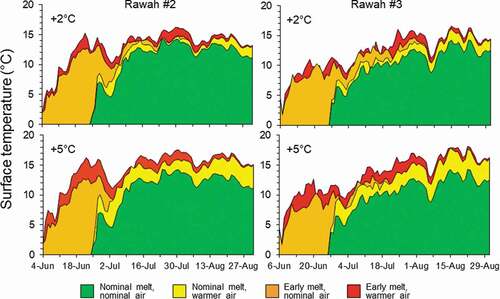
Figure 6. Predicted growing degree days in the study lakes under nominal conditions vs. increased air temperature and earlier snowmelt scenarios. Percentages show relative change from nominal conditions for the simulation period. Growing degree days extrapolated after 31 August until water temperature reached 4°C in autumn are also shown

Figure 7. Mean specific respiration rates of cutthroat trout and brook trout during ice-off to August 31 in Rawah #2 (A) and Rawah #3 (B) under six hydroclimate scenarios

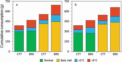
Figure 8. Predicted cumulative consumptive demand of cutthroat trout (CTT) and brook trout (BRK) in (a) Rawah #2 and (b) Rawah #3 during ice-off to 31 August across hydroclimate scenarios: nominal air temperatures and nominal snowmelt (green), nominal air temperatures and early snowmelt (orange), and the additional effect of 2°C (blue) and 5°C (red) warmer air temperatures on each snowmelt scenario