The effect of the second-order ionospheric term on GPS positioning in Antarctica

Figures & data

Figure 1. Geometry of the thin-layer model (not to scale). $R$ is the radius of the Earth, and $H$ corresponds to the height of the thin layer. Compared with $R$ and $H$, the height of Earth’s surface and antenna height are so small that they can be ignored. $z^{\prime }$ denotes the zenith angle at the IPP

Figure 2. $VTEC$ distribution 450 km above Antarctica at 0:00 UTC, 1 January 2012. One TEC unit (TECU) = 10¹⁶ electrons/m²

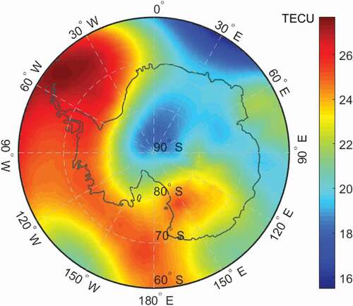
Figure 3. Geomagnetic field intensity distribution in Antarctica on 1 January 2012 450 km above the surface of the Earth, calculated based on IGRF-12. (a) Total intensity and (b)–(d) the field intensity in the x, y, and z, directions, respectively. The unit of geomagnetic field intensity is nano Tesla

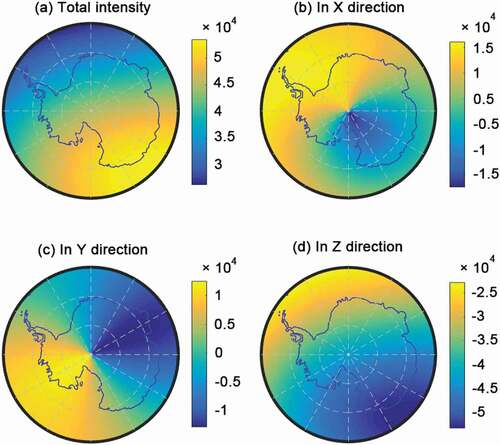
Figure 4. Antenna of continuously operating GPS system in Zhongshan Base, Larsemann Hills, East Antarctica. The GPS receiver type is LEICA GRX1200PRO, and the antenna type is LEIAT504

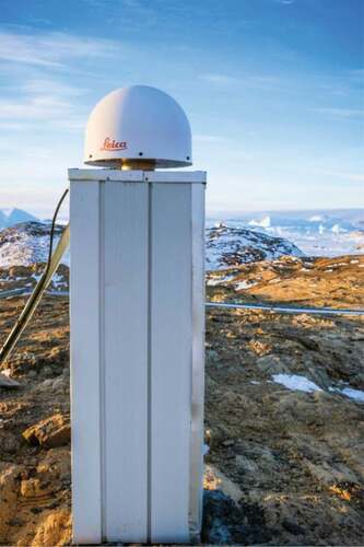
Figure 5. (a). Geographic distribution of the continuously operating GPS stations adopted in this study. Note that KUNL (Kunlun Base, China) is a summer station, only providing the data during January. (b). IPP distribution from 00:00 to 12:00 UTC on day 20120101

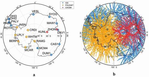
Figure 6. Flowchart of the data processing. TEQC (Translation, Editing, and Quality Check; Estey and Meertens 1999) and GPSTk (GPS Toolkit; Harris and Mach 2007) were used in the GPS preprocessing, and least squares estimation was undertaken in MATLAB software

Table 1. Mean values of GPS positioning errors in x, y, and z directions for each station derived by the second-order ionospheric term during the whole year for 2012 (mm)

Station name	Mean value yearly			Mean value in January			Mean value in July
	x	y	z	x	y	z	x	y	z
BERP	0.145	−1.316	1.583	0.280	−2.132	2.564	0.016	−0.399	0.474
CAS1	0.146	−1.589	1.839	0.195	−2.377	2.675	0.081	−0.622	0.770
CRDI	0.275	−0.279	1.292	0.504	−0.476	2.289	0.089	−0.076	0.318
DAV1	−0.141	−1.570	1.537	−0.222	−2.304	2.309	−0.051	−0.586	0.587
DUM1	−0.061	−1.203	1.798	−0.125	−1.783	2.606	−0.009	−0.491	0.786
JNSN	0.590	−0.802	1.451	0.811	−1.287	2.285	0.191	−0.215	0.361
KUNL	—	—	—	0.198	−1.286	3.023	—	—	—
LPLY	0.383	−1.067	1.244	0.717	−1.996	2.418	0.149	−0.338	0.417
MAW1	−0.419	−1.375	1.403	−0.573	−1.913	2.048	−0.146	−0.462	0.490
MCAR	−0.298	−0.907	1.590	−0.454	−1.304	2.465	−0.136	−0.349	0.550
MCM4	−0.230	−0.300	1.576	−0.187	0.221	2.188	−0.120	−0.145	0.617
OHI2	0.601	−0.618	1.067	0.973	−0.930	1.737	0.183	−0.213	0.367
OHI3	0.766	−0.595	1.119	1.246	−1.037	1.865	0.280	−0.154	0.384
PALM	0.759	−0.736	1.150	1.304	−1.265	1.977	0.259	−0.158	0.372
PALV	0.758	−0.718	1.158	1.299	−1.229	1.999	0.255	−0.158	0.375
RAMG	−0.091	−0.056	1.443	−0.006	−0.232	2.340	−0.055	0.037	0.487
ROTH	0.753	−0.796	1.225	1.303	−1.353	2.127	0.255	−0.223	0.370
SYOG	−0.412	−0.894	1.184	−0.496	−1.561	1.785	−0.144	−0.205	0.376
VESL	−0.083	−0.200	1.069	0.021	−0.422	1.778	−0.028	−0.012	0.327
WHTM	0.199	−0.846	1.549	0.423	−1.485	2.615	0.033	−0.198	0.431
ZHON	−0.138	−1.451	1.529	−0.234	−2.180	2.291	−0.048	−0.531	0.567
Total	0.175	−0.866	1.390	0.332	−1.349	2.256	0.053	−0.275	0.471

Note. Refer to Figure 5 for GPS station positions.

Figure 7. Time series of positioning errors derived by the second-order ionospheric term for twenty-one Antarctic GPS stations in 2012. Components x, y, and z represent the positioning errors in the east, north, and vertical directions, respectively

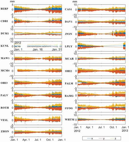
Figure 8. Yearly motion for each GPS station derived by the second-order ionospheric term. The arrows represent the size and direction of horizontal movement, and the depth of the color represents the size of the upward movement

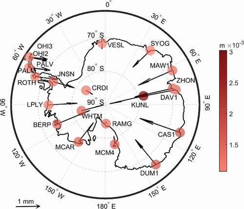
Figure 9. Average $VTEC$ values over all twenty-one stations for the year 2012. The time interval was set to every 2 hours

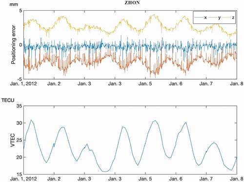
Figure 10. Relation of $VTEC$ and the positioning error for the first week of 2012. The top panel shows the effect of the second-order ionospheric term on GPS positioning in the x, y, and z directions at ZHON station. The bottom panel shows the average $VTEC$ values over the twenty-one stations

Estey, L. H., and C. M. Meertens. 1999. TEQC: The multi-purpose toolkit for GPS/GLONASS data. GPS Solutions 3 (1):42–49. doi:https://doi.org/10.1007/PL00012778.

 Web of Science ®Google Scholar

Harris, R. B., and R. G. Mach. 2007. The GPSTk: An open source GPS toolkit. GPS Solutions 11 (2):145–50. doi:https://doi.org/10.1007/s10291-006-0043-7.

 Google Scholar