A mild Younger Dryas recorded in southeastern Alaska

Figures & data

Figure 1. Location of study sites in southeastern Alaska: (1) Baker Island (this record); (2) Pass Lake, Prince of Wales Island (Ager and Rosenbaum 2009); (3) Mitkof Island (Ager et al. 2010); (4) Pleasant Island (Hansen and Engstrom 1996); (5) Lily Lake, Chilkat Peninsula (Cwynar 1990); (6) Haida Gwaii (Queen Charlotte Islands; Mathewes, Heusser, and Patterson 1993); (7) Haida Gwaii (Lacourse, Mathewes, and Fedje 2005); (8) Hummingbird Lake, Baranof Island (Ager 2019); (9) El Capitan Cave, Prince of Wales Island (Wilcox, Dorale, et al. 2019)

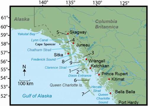
Figure 2. Bathymetry of Bonsai Lake with core site locations BBL4 and BBL6. Detailed analysis was only performed on BBL4

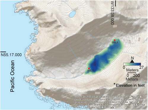
Figure 3. Sediment cores BBL4 and BBL6 from Baker Island showing lithologic changes and radiocarbon sampling sites

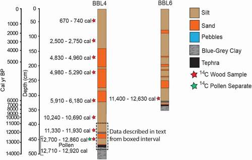
Table 1. List of radiocarbon dates on Baker Island

Sample location	Lab no.	Material	δ^13C(‰)	^14C age ± 1σ	±	Calibrated age	Median age (cal yr BP)^a
BBL4 55 cm	CAMS-168615	Wood	−25	780	30	669–740	700
BBL4 120 cm	CAMS-176643	Wood	−25	2,540	30	2,496–2,747	2,630
BBL4 180 cm	CAMS-171891	Wood	−25	4,305	35	4,831–4,961	4,860
BBL4 227 cm	CAMS-176642	Wood	−25	4,475	30	4,977–5,288	5,170
BBL4 320 cm	CAMS-171890	Wood	−25	5,230	45	5,911–6,177	5,990
BBL4 380 cm	CAMS-168618	Wood	−25	9,270	90	10,244–10,688	10,450
BBL4 422 cm	CAMS-176640	Wood	−25	10,065	50	11,332–11,929	11,610
BBL6 307 cm	CAMS-168582	Wood	−25	10,320	180	11,404–12,627	12,100
BBL4 455 cm	CAMS-169840	Pollen	−25	10,935	35	12,706–12,862	12,780
BBL4 455 cm	CAMS-168614	Wood	−25	10,955	35	12,712–12,916	12,790

Note. ^aCalibrated ages and median ages were calculated using 2σ range from IntCal13 (Reimer et al. 2013).

Figure 4. (A) Age–depth model fit in the Clam package in R (Blaauw 2010), based on simple linear interpolation between calibrated ages and extrapolated to a depth of 475 cm. The YD unit (Rasmussen et al. 2006) is highlighted in red. (B) Variable sedimentation rates based on age model in (A)

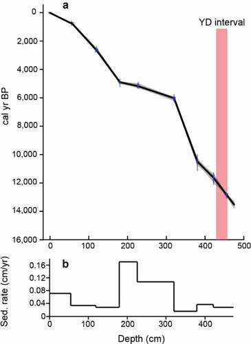
Figure 5. Pollen percentage and influx rates during the late Pleistocene. Mean grain size, magnetic susceptibility, percentage organics, C/N, δ¹³C, pollen zones, and CONISS cluster diagram are to the right of both pollen percentage and influx rates. The YD interval (Rasmussen et al. 2006) is bounded by red lines based on the ¹⁴C age model (see Figure 4)

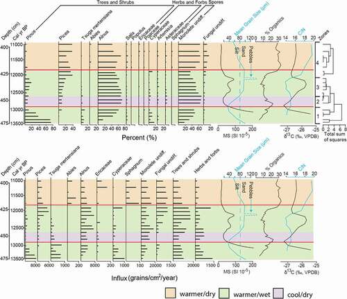
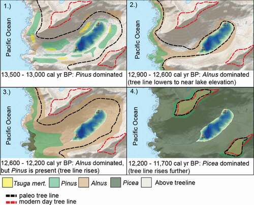
Figure 6. An interpretation of vegetation changes based on data from Figure 5 at distinct time intervals leading up to and during the YD chronozone

Ager, T. A., and J. G. Rosenbaum. 2009. Late glacial-Holocene pollen-based vegetation history from Pass Lake, Prince of Wales Island, southeastern Alaska. US Geological Survey Professional Paper 1760–G.

 Google Scholar

Ager, T. A., P. E. Carrara, J. L. Smith, V. Anne, and J. Johnson. 2010. Postglacial vegetation history of Mitkof Island, Alexander Archipelago, southeastern Alaska. Quaternary Research 73:259–68. doi:https://doi.org/10.1016/j.yqres.2009.12.005.

 Google Scholar

Hansen, B. C. S., and D. R. Engstrom. 1996. Vegetation history of Pleasant Island, southeastern Alaska, since 13,000 yr B.P. Quaternary Research 46:161–75. doi:https://doi.org/10.1006/qres.1996.0056.

 Web of Science ®Google Scholar

Cwynar, L. C. 1990. A late Quaternary vegetation history from Lily Lake, Chilkat Peninsula, southeast Alaska. Canadian Journal of Botany 68:1106–12. doi:https://doi.org/10.1139/b90-139.

 Google Scholar

Mathewes, R. W., L. E. Heusser, and R. T. Patterson. 1993. Evidence for a Younger Dryas-like cooling event on the British Columbia coast. Geology 21:101–04. doi:https://doi.org/10.1130/0091-7613(1993)021<0101:EFAYDL>2.3.CO;2.

 Web of Science ®Google Scholar

Lacourse, T., R. W. Mathewes, and D. W. Fedje. 2005. Late-glacial vegetation dynamics of the Queen Charlotte Islands and adjacent continental shelf, British Columbia, Canada. Palaeogeography, Palaeoclimatology, Palaeoecology 226:36–57. doi:https://doi.org/10.1016/j.palaeo.2005.05.003.

 Web of Science ®Google Scholar

Ager, T. A. 2019. Late Quaternary vegetation development following deglaciation of northwestern Alexander Archipelago, Alaska. Frontiers in Earth Science 7:104. doi:https://doi.org/10.3389/feart.2019.00104.

 Web of Science ®Google Scholar

Wilcox, P. S., J. A. Dorale, J. F. Baichtal, C. Spötl, S. J. Fowell, L. R. Edwards, and J. L. Kovarik. 2019b. Millennial-scale glacial climate variability in Southeastern Alaska follows Dansgaard-Oeschger cyclicity. Scientific Reports 9 (1):1–8. doi:https://doi.org/10.1038/s41598-019-44231-1.

 Google Scholar

Reimer, P. J., E. Bard, A. Bayliss, J. W. Beck, P. G. Blackwell, C. B. Ramsey, C. E. Buck, H. Cheng, R. L. Edwards, M. Friedrich, et al. 2013. IntCal13 and Marine13 radiocarbon age calibration curves 0–50,000 years cal BP. Radiocarbon 55 (4):1869–87. doi:https://doi.org/10.2458/azu_js_rc.55.16947.

 Web of Science ®Google Scholar

Blaauw, D. 2010. Clam version 2.2. Accessed November 11, 2016. http://www.chrono.qub.ac.uk/blaauw/clam.html.

 Google Scholar

Rasmussen, S. O., K. K. Andersen, A. M. Svensson, J. P. Steffensen, B. M. Vinther, H. B. Clausen, M. L. Siggaard‐Andersen, S. J. Johnsen, L. B. Larsen, D. Dahl‐Jensen, et al. 2006. A new Greenland ice core chronology for the last glacial termination. Journal of Geophysical Research: Atmospheres 111 (D6). doi:https://doi.org/10.1029/2005JD006079.

 Google Scholar