Timing of Little Ice Age maxima and subsequent glacier retreat in northern Troms and western Finnmark, northern Norway

Figures & data

Figure 1. Study area location in Troms and Finnmark county, northern Norway. The white rectangle represents the area under investigation, defined as “Region 3–Troms North,” and the gray rectangle shows “Region 2–Øksfjord” (Andreassen, Winsvold, et al. 2012). Turquoise rectangles indicate the three glacial regions, defined as A, B, and C (the Bergfjord Peninsular). The yellow rectangle shows the location of the field site within the Rotsund Valley. The location of the Rotsundelv churchyard (RC) and Storslett churchyard (SC) used for lichenometric dating controls are highlighted along with the location of the weather station at Sørkjosen Airport (SA). Note: The base image is a 2018 pan-sharpened Landsat 8 scene displayed as a false color composite; red–green–blue as 5-4-3

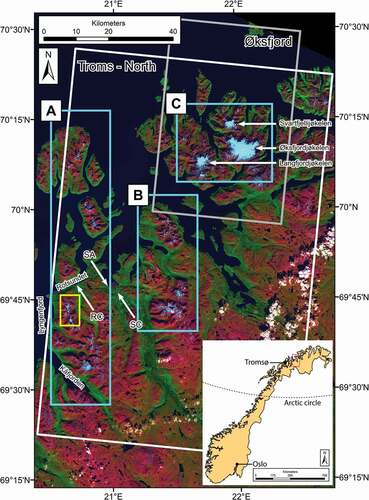
Figure 2. (A) 2016 Aerial orthophotographs (NORGEiBILDER 2019) of the Rotsund Valley field site. Photographs of the four glaciers visited in the field: (B) 115, (C) 117, (D) 121, and (E) 123. The dashed red line denotes the glacier extent in 2018

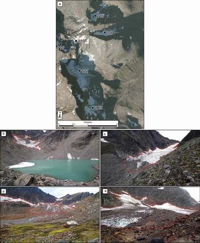
Figure 3. Geomorphological map of the field site within the Rotsund Valley (location shown in Figure 1) showing glaciers 115, 117, 118, 119, 121, and 123. Map based on field mapping and aerial orthophotographs (image date 16 September 2016) with 0.25 m spatial resolution

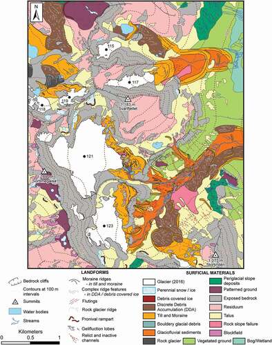
Figure 4. Part of a Norwegian Mapping Authority 1:50,000 topographic map (map sheet: 1634 II) showing the digitized 1953 glacier outlines (turquoise) in the Rotsund Valley (yellow box in Figure 1). The 2001 Andreassen, Winsvold, et al. (2012) glacier outlines (black) are overlaid, with IDs shown. The red boxes highlight seven glaciers in this area that were not included on the 1953 topographic map. The two purple outlines are snow patches mapped in Andreassen, Winsvold, et al. (2012), one of which was initially mapped as a glacier on the 1953 map. Glaciers 115, 117, 121, and 123 are seen in Figure 3. For scale, grid squares are 1 × 1 km

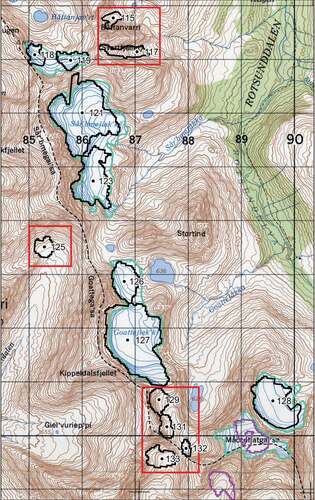
Figure 5. Example of the LIA moraine examined in the field (foreland of glacier 121) that can be seen from (A) aerial orthophotograph (0.25 m resolution; NORGEiBILDER 2019) and (B) oblique photograph. The M1 moraine is sharp crested, with little evidence of slumping, predominantly unaffected by periglacial slope activity, and on the distal side of the moraine there is a distinct vegetation trimline. Note: The LIA moraines shown on the aerial imagery are not easily distinguishable on the 15 m Landsat imagery and not identifiable on the 30 m Landsat imagery

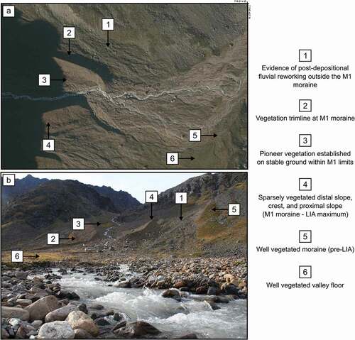
Table 1. Lichen size data (single largest lichen and mean of the 5LL) from the moraines within the four glacial forelands of the field site. Glacier IDs are provided as assigned within the Inventory of Norwegian Glaciers (Andreassen, Winsvold, et al. 2012)

Glacier ID	Moraine elevation (m a.s.l.)	Assigned moraine ID	Single largest lichen (mm)	5LL (mm)
115	660–690	M1	38	37.4
117	570–600	M1	35	33.2
	560–580	M2	32	26.5
	560–570	M3	24	23
121	340–440	M1	41	37
	360–380	M2	27	27
	595	M3	24	23.4
	545	M6	9	8.2
	555	M7	6	5.2
	570	M8	0	0
123	440–450	M1(1)	42	35.6
	425–500	M1(2)	35	33
	455–510	M2	30	23.6
	550–570	M4	14	13.2
	570	M5	13	11.2
	545–600	M6	8	7.4
	550	M8	0	0

Table 2. Results of the lichenometric dating providing calculated ages for the moraines under investigation

Glacier ID	Moraine	5LL (mm)	Calculated age (years before 2018)	Calculated age ±20% (years before 2018)	Date	Date ±20%
115	M1	37.4	204	245–163	1814	1773–1855
117	M1	33.2	143	172–114	1875	1846–1904
	M2	26.5	82	98–66	1936	1920–1952
	M3	23	61	73–48	1957	1945–1970
121	M1	37	196	235–157	1822	1783–1861
	M2	27	85.8	103–69	1932	1915–1949
	M3	23.4	63	76–50	1955	1942–1968
	M6	8.2	18	22–14	2000	1996–2004
	M7	5.2	14	17–11	2004	2001–2007
	M8	0	9	11–7	2009	2007–2011
123	M1(1)	35.6	175	175–140	1843	1808–1878
	M1(2)	33	140.5	169–112	1877	1849–1906
	M2	23.6	64	79–51	1954	1939–1967
	M4	13.2	27	32–22	1991	1986–1996
	M5	11.2	23	28–18	1995	1990–2000
	M6	7.4	17	20–14	2001	1998–2004
	M8	0	9	11–7	2009	2007–2011

Figure 6. Lichenometric dating curve constructed from lichen growth on dated headstones within the Rotsundelv and Storslett churchyards. The black line represents a logarithmic curve fitted to the largest lichens, and the dotted gray lines represent standardized ±20 percent lichenometric error margins. The curve has been extrapolated to represent lichen growth over the past 210 years

Figure 7. Geomorphological mapping of glacier 115 foreland; (A) aerial orthophotographs (NORGEiBILDER 2019; image date 19 September 2011) with 0.25 m spatial resolution showing the glacier foreland, (B) Geomorphological map of area shown in (A) showing the foreland of glacier 115 (Figure 2b) with annotations showing the moraine surveyed for lichenometry and the resulting calculated ages. Note:  Map based on field mapping and aerial orthophotographs from 2016 however, due to shading on the 2016 imagery on which the geomorphological map (B) is based, aerial imagery from 2011 (A) is shown

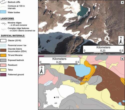
Figure 8. Geomorphological mapping of glacier 117 foreland; (A) aerial orthophotographs (image date 19 Septemeber 2011) with 0.25 m spatial resolution showing the glacier foreland, (B) Geomorphological map of area shown in (A) showing the foreland of glacier 117 (Figure 2c) with annotations showing the moraine surveyed for lichenometry and the resulting calculated ages. Note: Map based on field mapping and aerial orthophotographs from 2016 however, due to shading on the 2016 imagery on which the geomorphological map (B) is based, aerial imagery from 2011 (A) is shown

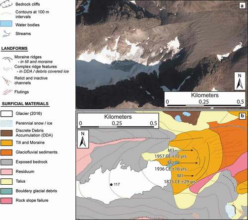
Figure 9. Geomorphological mapping of glacier 121 foreland; (A) aerial orthophotographs (image date 16 September 2016) with 0.25 m spatial resolution showing the glacier foreland, (B) Geomorphological map of area shown in (A) showing the foreland of glacier 121 (Figure 2d) with annotations showing the moraine surveyed for lichenometry and the resulting calculated ages. Map based on field mapping and aerial orthophotographs from 16 September 2016 with 0.25 m spatial resolution

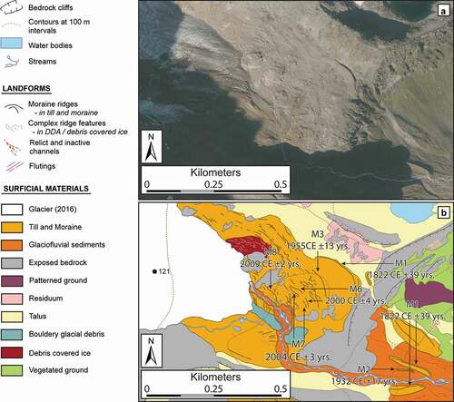
Figure 10. Geomorphological mapping of glacier 123 foreland; (A) aerial orthophotographs (image date 19 September 2011) with 0.25 m spatial resolution showing the glacier foreland, (B) Geomorphological map of area shown in (A) showing the foreland of glacier 123 (Figure 2e) with annotations showing the moraine surveyed for lichenometry and the resulting calculated ages. Note: Map based on field mapping and aerial orthophotographs from 2016 however, due to shading on the 2016 imagery on which the geomorphological map (B) is based, aerial imagery from 2011 (A) is shown

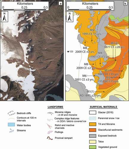
Figure 11. Oblique aerial photographs taken on (A) 8 March 1952 and (C) 31 July 1952 and alongside a zoomed and cropped copy of the aforementioned images (B) and (D). Glaciers are labeled according to the Andreassen, Winsvold, et al. (2012) glacier IDs. The dashed lines outline the visible moraines investigated in this study and the blue arrows in (B) show where glaciers were confluent with adjoining glaciers/ice bodies. Image source: National Library of Norway (2019)

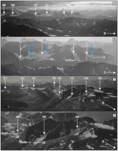
Figure 12. Comparisons of glacial area change between LIA maximum and 1989/2018

Figure 13. Overview of glacier area change from our Rotsund field site since LIA maximum until 2018 (based on moraine maps and lichenometric dating) and including glacier outlines from 1956 topographic maps. The background image is the Norwegian Mapping Authority N50 Digital Terrain Map (NORGEiBILDER 2019)

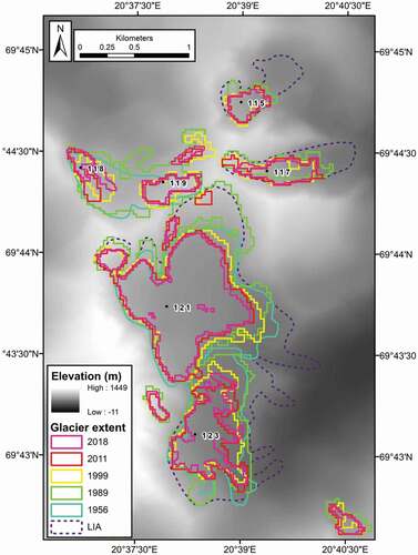
Table 3. Summary of remotely sensed glacier area measurements and size over the study period for the whole region of investigation

Year	1989	1994	1999	2006	2011	2014	2018
No. of glaciers	219	228	237	243	249	249	252
Total area (km^2)	101.8	96	81.9	81.9	73.7	67.1	66.4
Max. glacier area (km^2)	12.7	12.5	12.4	12.4	12	11.8	11.8
Mean glacier area (km^2)	0.46	0.42	0.35	0.34	0.3	0.27	0.26
No. glaciers ≥0.5 km^2 (%)	18	16	13	12	10	7	8
No. glaciers <0.5 km^2 (%)	82	84	87	88	90	93	92
Total area change (km^2)^a	n/a	−5.8	−14.1	−0.03	−8.9	−6.6	−0.8
Total area change (%)^a	n/a	−6	−15	−0.04	−10	−9	−1
No. of certain glaciers	164	167	163	169	174	179	182
Total area (km^2)	96.6	91.4	79	78.7	71.6	65.2	64.6
Max. glacier area (km^2)	12.7	12.5	12.4	12.4	12	11.8	11.8
Mean glacier area (km^2)	0.59	0.55	0.48	0.47	0.41	0.36	0.36
No. glaciers ≥0.5 km^2 (%)	24	22	19	17	15	10	11
No. glaciers <0.5 km^2 (%)	76	78	81	83	85	90	89
Total area change (km^2)^a	n/a	−5.2	−12.4	−0.28	−7.1	−6.4	−0.64
Total area change (%)^a	n/a	−5	−14	−0.4	−9	−9	−1
No. of probable glaciers	10	9	9	9	11	15	13
Total area (km^2)	1.3	0.81	0.43	0.37	0.37	0.42	0.36
Max. glacier area (km^2)	0.33	0.26	0.2	0.17	0.08	0.04	0.04
Mean glacier area (km^2)	0.13	0.09	0.05	0.04	0.03	0.03	0.03
Total area change (km^2)^a	n/a	−0.52	−0.38	−0.06	0	+0.05	−0.06
Total area change (%)^a	n/a	−39	−47	−14	0	+13	−14
No. of possible glaciers	45	52	65	65	64	55	57
Total area (km^2)	3.9	3.8	2.5	2.8	2	1.5	1.5
Max. glacier area (km^2)	0.3	0.29	0.21	0.21	0.13	0.08	0.07
Mean glacier area (km^2)	0.09	0.07	0.03	0.04	0.03	0.03	0.03
Total area change (km^2)^a	n/a	−0.09	−1.27	+0.31	−0.81	−0.5	+0.03
Total area change (%)^a	n/a	−2	−34	+13	−29	−25	+2

Note. ^aArea change based on the difference between the total area mapped at the previous time step.

Figure 14. Plots of glacier area and length reduction, as both absolute and percentage values, between the periods (A), (B) LIA to 1989 and (C), (D) 1989 to 2018. Note: The blue circles and corresponding text represent glaciers with at least one proglacial lake within the LIA moraine limits and the numbers represent the individual glacier IDs (Andreassen, Winsvold, et al. 2012)

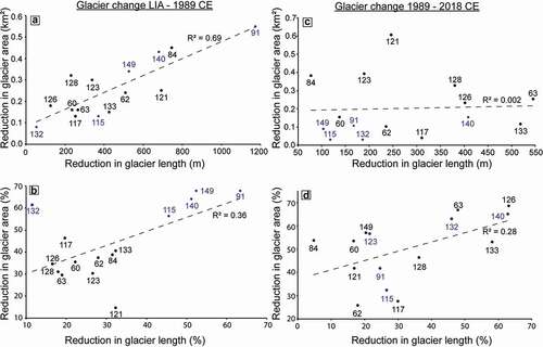
Figure 15. Comparisons of glacier area change between individual sets of historic outlines (from 1:100,000 Gradteigkart [1907 map] and 1:50,000 Norwegian Mapping Authority topographic maps [1966, 1952, 1954, 1955, and 1956 maps]) and our remotely sensed outlines from 1989. Note: Only the outlines in panel I are overlapping outlines from different time steps; the remaining panels II–V represent glacier outlines from different areas within northern Troms at separate time steps (historic outlines from Winsvold, Andreassen, and Kienholz [2014])

Figure 16. (A) Mean annual temperature, (B) mean summer (June–September) temperature, and (C) mean winter (October–May) temperature. Smoothed dark red and blue lines represent ten-year average; dashed line in (C) represents 0°C. Data recorded in Tromsø from two independent weather stations #90440 and #90450 that have been combined to make a continuous record since 1870 (see section Little Ice Age maxima to late twentieth century; accessed via eKlima 2019)

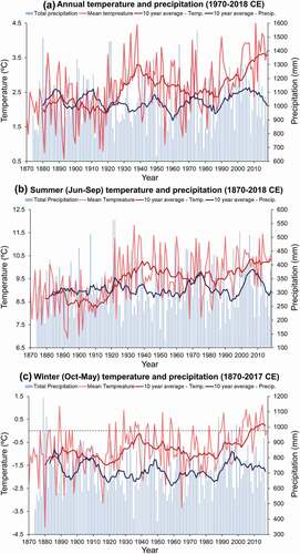
Figure 17. Color-coded map of absolute glacier area change (km²) from 1989 to 2018. Panels 1, 2, and 3 show the predominantly glaciated parts of areas A, B, and, C as outlined in Figure 1

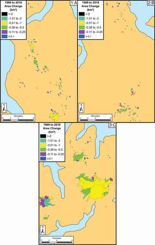
Figure 18. Color-coded map of relative glacier area change (percentage) from 1989 to 2018. Panels 1, 2, and 3 show the predominantly glaciated parts of areas A, B, and C as outlined in Figure 1

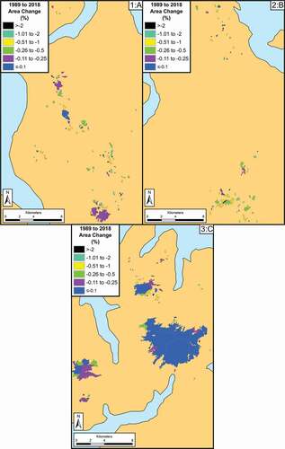
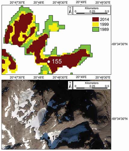
Figure 19. An example of glacier fragmentation over time. (A) Glacier 155 mapped as one unit in 1989. By 1999 it has shrunk and fragmented into two units; the main body and an isolated (glacier) ice patch from its central tongue. In 2014 the glacier had fragmented into three separate units and the ice patch has shrunk below the 0.01 km² size threshold. (B) Aerial orthophotograph (image taken on 16 September 2019 with 0.25 m resolution; NORGEiBILDER 2019) showing glacier 155 in 2016. Note: Though it is possible to discern the very small glacier fragment that shrank below the 0.01 km² size threshold on the aerial imagery (0.25 m resolution), it was not possible to accurately map it on the satellite imagery (15 m resolution)

Andreassen, L. M., S. H. Winsvold, F. Paul, and J. E. Hausberg. 2012. Inventory of Norwegian glaciers, ed. L. M. Andreassen and S. H. Winsvold. Oslo: Norwegian Water Resources and Energy Directorate.

 Google Scholar

NORGEiBILDER. 2019. Norwegian Mapping Authority. Available at: http://www.norgeibilder.no.

 Google Scholar

National Library of Norway. 2019. Pictures. Available at: https://www.nb.no/search?q=wider%C3%B8e%20nordreisa&mediaQ25 type=bilder&fromDate=19500101&”toDate=19531231

 Google Scholar

Winsvold, S. H., L. M. Andreassen, and C. Kienholz. 2014. Glacier area and length changes in Norway from repeat inventories. Cryosphere 8 (5):1885–903. doi:https://doi.org/10.5194/tc-8-1885-2014.

 Web of Science ®Google Scholar

eKlima. 2019. Norwegian Meteorological Institute climate database. Available at: http://www.eklima.no/.

 Google Scholar