
Figures & data
Figure 1. The Diminishing Real Estate Model (DREM). The alpine biota (shaded band) undergoes two climate regimes. Upper left: At T1, cool adapted alpine biota occupy a broadly connected area of the mountain scape during cool climates. At T2, the climate has warmed, displacing and isolating the alpine habitat on separate peaks of the same mountain scape. The alpine habitats represent two frustums (conic sections) whose surface area can be calculated (center left column). Note that both frustum depths remain uniform while the radii reduce. Under the DREM, several ecological outcomes are possible across generation time (center right column). Within alpine habitats, community ecology indices are expected to have characteristic curves (colored lines) with increased elevation and, all things being equal, respond monotonically to climate warming (red) or cooling (blue). The model assumes typical species–area curves with the formula for a single mountain analogous to the island biogeography area curve: S= CAz, where S is the number of species, A is the area of frustum, and c and z are fitted intercepts
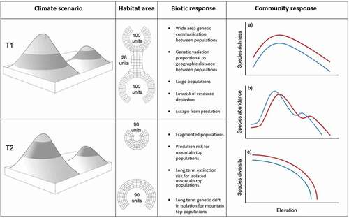
Figure 2. Map showing central Southern Alps of the South Island, Aotearoa/New Zealand, with additional mountain ranges labeled. Snow crystal icons show large regions of present-day glaciation. Dark blue dots are the end of summer snow line index glaciers (n = 50) including potential locations for establishing Climate Monitoring Units (CMUs), indicated in light blue. Brewster Glacier and French Ridge are marked in red
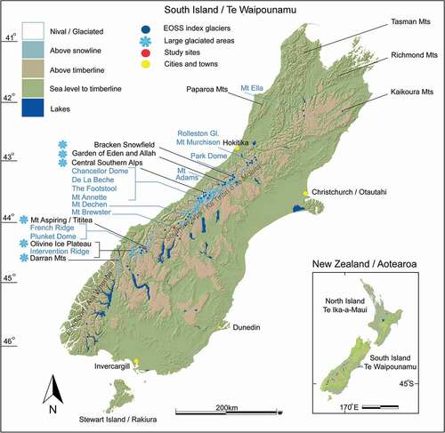
Table 1. Potential responses of, and effects on, alpine invertebrate populations to a predicted rise in elevation of optimal habitat conditions, driven by a warming climate in the Southern Alps of New Zealand
Figure 3. A typical End of Summer Snow line (EOSS) on the Rolleston Glacier, a very small cirque-type glacier in Arthur’s Pass National Park, Southern Alps. The glacier albedo acts to thermally buffer winter snow, which ablates slowly from the glacier snout at the onset of summer. The highest elevation of the snow line represents the average of all ablation sources and provides a relative position for the upper boundary isotherm of the alpine zone. Two snow patches are visible either side of the massif indicating that even under high Infra–Red radiation (from scree and rock) the snow line remains detectable
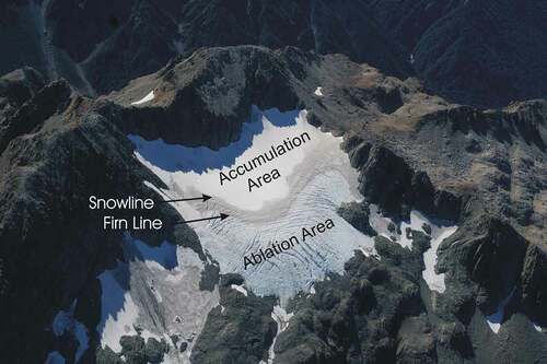
Table 2. Characteristics of the Southern Oscillation Index (SOI) and effects on New Zealand weather and snow line elevation in the Southern Alps
Figure 4. Composite images of the two sampling locations, Brewster Glacier (a-d) and French Ridge (e-h). Both sites support an ecologically isolated biota, confined to a ridge and extending from the timberline to the permanent snowline (or mountain summit). (a) Map of the Brewster Glacier and environs (Topomap 1:50 000 Series). Red line depicts invertebrate sampling transect, grid squares=1km. (b) aerial photograph of Brewster Glacier in 2016, view toward south west. (c) Typical snowline aerial photograph of Brewster Glacier showing firn line and End Of Summer Snow line (EOSS) with sampling transect (red line). (d) Ground view of Mt Brewster taken from transect line. Image insert is a female Pharmacus brewsterensis: Rhaphidophoridae, a resident of this habitat. (e) Map of French Ridge, Mt Aspiring/Tititea National Park (Topomap 1:50 000 Series). Red line depicts invertebrate sampling transect. Grid squares=1km. (f) Aerial photograph of French Ridge (showing transect) and Bonar Glacier. (g) View looking up to Mt French, from 1800 m a.s.l. Tapering red line represents transect path. Insert image shows the scree weta Deinacrida connectens feeding (at night) on a native Ranunculus herb. (h) Down-slope view of French Ridge showing hut location, sampling transect and example of alpine herb field/stone pavement
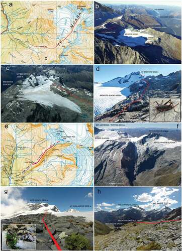
Table 3. Summary data for fifty snow line index glaciers in the Southern Alps, New Zealand. Glaciers are listed geographically from north to south
Figure 5. Model of upslope habitat tracking by an Alpine Invertebrate Biota (AIB). Colored temperature ellipses represent populations of different species and their optimal (realized) niche elevation. Densities are represented by three median width classes. The diagram shows an upslope shift of 120 m by the End of Summer Snow line (EOSS) between 1977 (T1) and 2017 (T2), a response correlated with atmospheric warming. T2 populations located at, near, or even extending into the previous snow line are assumed to have tracked up slope since T1. Populations can be directly sampled today for occupancy on snow- and ice-free slopes at T2. Nine populations protrude above the T1 snow line (blue dashes). For the remaining populations, upslope tracking has occurred if their T2 median densities are at elevations previously cooler than today’s apparent optimal temperatures, given a lapse rate of 6.6°C km−1 relative to the snow line. The “red” population provides an example; at T2 the highest population density is located at 1,520 m a.s.l., with an isotherm of 3.6°C. Forty years ago, the same isotherm was 120 m lower
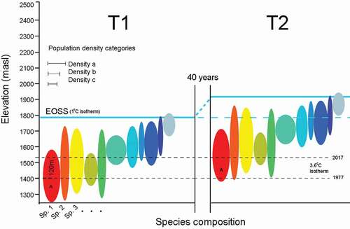
Table 4. Site selection criteria for establishing Climate Monitoring Units (CMUs) and measuring upslope tracking of the End of Summer Snow line (EOSS) by alpine invertebrates in the Southern Alps of New Zealand
Table 5. Checklist of alpine invertebrate taxa from Brewster Glacier and French Ridge, considered as members of the Alpine Invertebrate Biota (AIB). Maximum counts per elevation (at T2) are listed
Figure 6. Alpine invertebrate species abundance plots for (a) Brewster Glacier (n = 29) and (b) French Ridge (n = 25). Data are total individual counts per taxon; elevation range was from 1,400 to 2,200 m a.s.l. Both locations generated characteristic curves, with few taxa represented by many individuals and many with few counts. Grasshoppers represent the majority of alpine invertebrate biomass, probably reflecting the density of snow tussock (Chionochloa sp.)
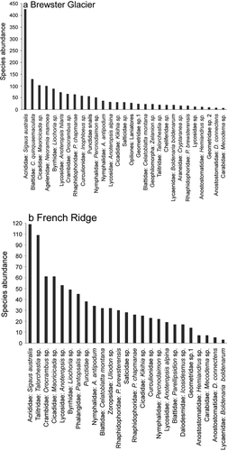
Figure 7. Species richness curves (number of taxa) per 100-m contour for (a) Brewster Glacier and (b) French Ridge. Both locations show strong negative trends. For Brewster Glacier, a fourth-order polynomial curve provided the best fit (R2 = 0.965). Taxon richness peaked at around 1,600 m a.s.l., declining by approximately five taxa per 100-m upslope shift. For French Ridge the best-fit trace was linear, with a strong negative trend (R2 = 0.947). French Ridge taxon richness declined at 2.7 taxa per 100 m of elevation gain
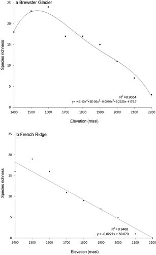
Figure 8. Violin plots showing relative densities of invertebrate populations for T2 (March 2016) at (a) Brewster Glacier and (b) French Ridge. Black dots are population medians; horizontal blue lines are snow lines (T1 and T2). Any taxa extending above the snow line were present either on snow or basking on rock outcrops close to the 2016 snow line. Colors are representative of woody shrubland (green), snowgrass (beige), and rock/snow (blue). Above 1,800 m a.s.l. the alpine habitat comprised short-horned grasshoppers (Acrididae), cave weta (Rhaphidophoridae), and free-living alpine wolf spiders (Anoteropsis alpina)
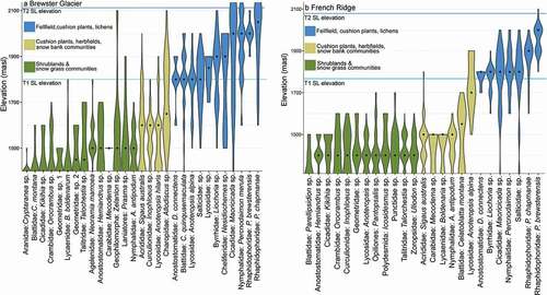
Figure 9. Graph showing elevations for the end of summer snow line (upper blue line) and timberline (lower green) plotted against latitudinal distance from the Kaikoura Mountains to Fiordland. Data are from fifty index glaciers in the Southern Alps of New Zealand and monitored between 1977 and 2016. Timberlines derived from 1:50,000 topographic maps. The snow line and timberline descend at approximately 130 m per degree of latitude (data from Willsman, Chinn, and Macara Citation2015, Citation2017). Colored shading represents our definition of the alpine zone and the region inhabited by the Alpine Invertebrate Biota (AIB), indicated as invertebrate silhouettes. Skyline trace shows high point elevations of mountains at specific distances from origin
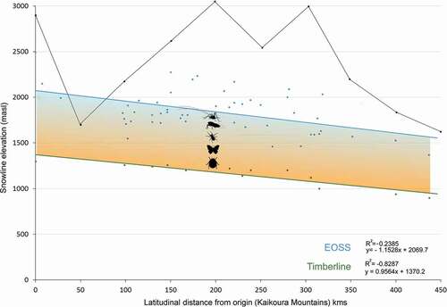
Figure 10. Combination graph showing a relationship between actual End of Summer Snow line (EOSS) data (blue line) and the Southern Oscillation Index (SOI), sea level air pressure anomaly as fluctuating red line. The ascending linear blue line traces the least-squares fit for the EOSS data. The red line trace shows an increase of the SOI over the same period. Here, the snow line rises at 3.10 m a−1 with a 0.144 correlation coeffcient (significantly greater than zero). The EOSS was correlated with SOI fluctuations (Kolmogorov-Smirnov test: D = 0.5, p = 0.1678). Positive SOI values represent La Niña weather anomalies and negative values represent the El Niño system
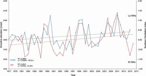
Figure 11. Local End of Summer Snowline (EOSS) plots for each sampling site. Upper plot: Snowline rise for Brewster Glacier showing a rate of 5.73m a-1 (y5.7438x -9549.8 = 2023m–1811m a-38). The positive correlation (0.43) was significant: t(34) = 22.2715, p < 0.05, x̄ = 1923, σ = 157.88 (R2 = 0.16). Lower plot: Snowline rise over 35 years for the Findlay Glacier (nearest analogue to French Ridge) showing a rate of 4.45m a-1, between years 1981 and 2016. The positive correlation (0.40) was significant: t(32)=22.2715, p < 0.05, x̄ = 1690, σ = 101.82 (R2 = 0.1531)
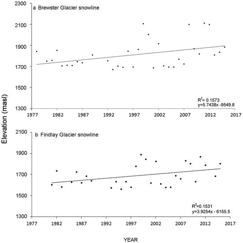
Figure 12. A synthesis of the model. Each graph shows four variables: The End of Summer Snow line (EOSS), the Alpine Invertebrate Biota (AIB, on abscissa), two time periods, and the two sites (a) Brewster Glacier and (b) French Ridge. Blue and yellow lines represent observed and calculated population density–elevation values, respectively. Snow line elevations are shown by the two horizontal blue lines for T1 and T2. For Brewster Glacier the snow line has risen 220 m, with seven taxa occupying slopes previously under the end of summer snow line some thirty-eight years ago (actual tracking). Six of those taxa had medians located at 1,800 m a.s.l. and two were measured at about the T2 snowline (1,910 m a.s.l.). This suggests that those taxa have actively tracked the snow line but not necessarily at the same rate. By contrast, the modelled tracking rise shows a considerably greater increase (up to 600 m) in elevation of populations over the same time period. The French Ridge (Findlay Glacier) snow line elevation shift was 160 m between T1 and T2. Lower elevation taxa potentially shift further with a rising snow line, whereas high elevation taxa are confined to a narrow thermal zone. The area between the taxa elevations is suggestive of a hysteresis function. See Discussion for details
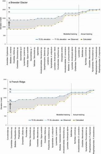
Table 6. List of Southern Alps locations with potential for establishing Climate Monitoring Units (CMUs). Each location has a corresponding index glacier (within 8 km of the monitoring site), which can provide End of Summer Snow line (EOSS) elevation data
Table 7. Candidate invertebrate taxa for monitoring alpine ecosystem condition within Ecological Management Units (EMUs) and Climate Monitoring Units (CMUs). Taxa are common to the New Zealand Southern Alps