Figures & data
Table 1. Lake morphometry and catchment characteristics of study lakes. Vegetation coverage was calculated from 2009 land cover data with a 30-m resolution from the CSC2000 v database (Center for Topographic Information, Earth Sciences Sector and Natural Resources Canada Citation2009). Glacial coverage was based on the Randolph Glacier Inventory (RGI Consortium Citation2017)
Figure 1. Topographic map of Lake O’Hara catchment showing study lakes and major land cover characteristics. Land cover delineation was based on 2006 aerial photography; current glacial extents are smaller than indicated on the map. Gaps in streams represent reaches of subsurface flow
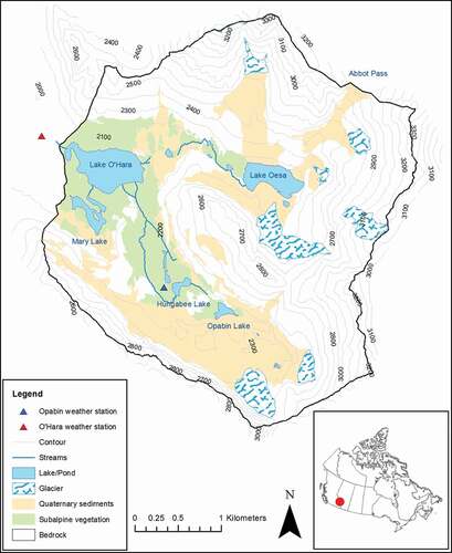
Figure 2. Plot of Kd320 (m−1) vs. time in the four study lakes over thirteen years (2006–2018). Lake O’Hara has no value for 2011
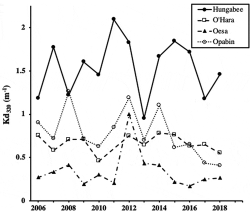
Figure 3. Correlograms for correlation coefficients between Kd320 (m−1) and cumulative precipitation (mm) for increasing periods of time preceding sampling in (a) Lakes Hungabee and O’Hara and (b) Lakes Oesa and Opabin. Correlations were calculated for fifteen-day increments of cumulative precipitation. Coefficients above the solid horizontal lines were significant (p < .05)
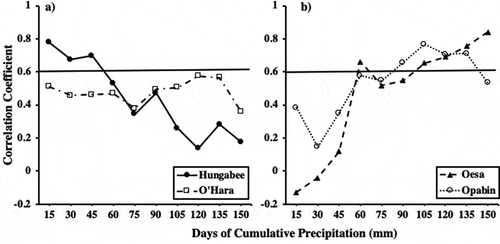
Figure 4. Scatterplots of Kd320 (m−1) vs. cumulative precipitation (mm) in (a) Hungabee for the 15 days preceding sampling, (b) Opabin for the 105 days preceding sampling, and (c) Oesa for the 150 days preceding sampling. Each scatterplot represents the strongest correlation observed in each study lake. No scatterplot is presented for O’Hara because no correlations were significant in this lake
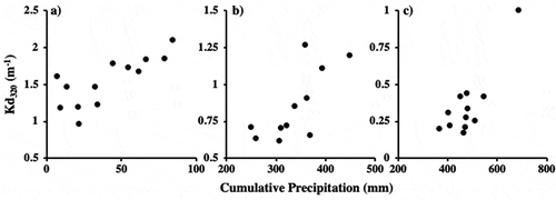
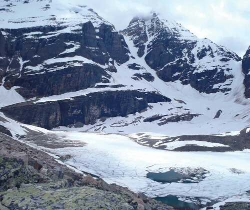
Figure 5. Photo of Lake Oesa on 2 July 2012 showing avalanche debris on ice surface below Abbott Pass. Photo was taken by MHO