Warmer temperatures promote shrub radial growth but not cover in the central Canadian Arctic

Figures & data

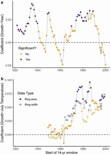
Figure 1. (a) The location of Walker Bay and potential sources of climate data in the central Canadian Arctic, (b) the location of our sampling plots at Walker Bay, (c) an image of a Salix richadsonii shrub at Walker Bay, and (d) an example of a stained cross section. There was one shrub sampled in 2010 from a snap-trap transect hidden by the legend in (b). Photo credit: Angélique Dupuch and Clara Morrissette-Boileau

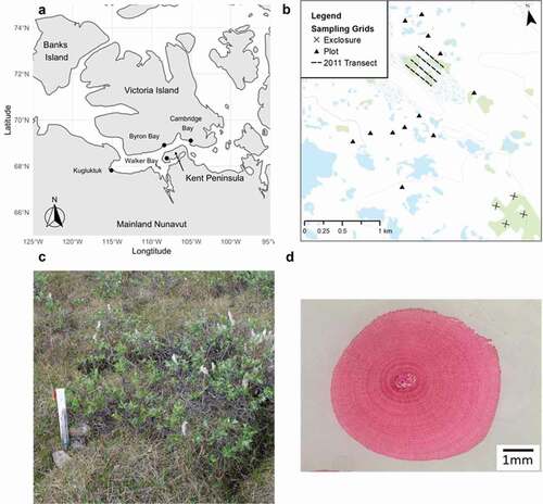
Figure 2. The trend in mean (a) annual temperature and (b) July temperature at the Cambridge Bay Airport since 1949 (data from Environment Canada’s weather station at Cambridge Bay, approximately 150 km northeast of the field site); Blue lines are predicted from linear models using the full data set, and orange data points represent the data from 1996 to 2010 (no significant regressions: [a] p = .65; [b] p = .39) when we have shrub cover estimates

Figure 3. Standardized ring width chronology built from fifty-four Salix richardsonii shrubs from Walker Bay, Nunavut, Canada. The number of individual shrubs (sample depth) that contribute to each point in the chronology is indicated by the filled polygon (minimum = one shrub from 1922 to 1924)

Figure 4. The response function coefficients for the annual growth (estimated as the standardized ring width) of Salix richardsonii and (a) mean monthly temperature and (b) total monthly precipitation from 1949 until 2013. Lowercase letters on the horizontal axis denote the months in the year before growth; uppercase letters refer to months in the year of growth. Black points represent statistically significant response function coefficients. Dashed lines and open symbols represent an analysis using the data from 1996 to 2010, which is the same period for which we have shrub cover data. We could only conduct the 1996 to 2010 analysis from March to September of the growth year because there were only fourteen available degrees of freedom for seven months each with two climate variables

Figure 5. (a) The trend in average ring area over time and its (b) relationship with July temperature. Ring area significantly increased over time and was significantly correlated with July temperature. Blue lines are predicted from linear models using the full data set, and orange points and lines use the data from 1996 to 2010 when we have shrub cover estimates (there was no significant relationship between ring area and year in the restricted data set; p = .74). The range in (a) and error bars in (b) show ±1 standard deviation in ring area truncated at zero. The sample depth for the ring area chronology (a) is the same as the ring width chronology (Figure 2)

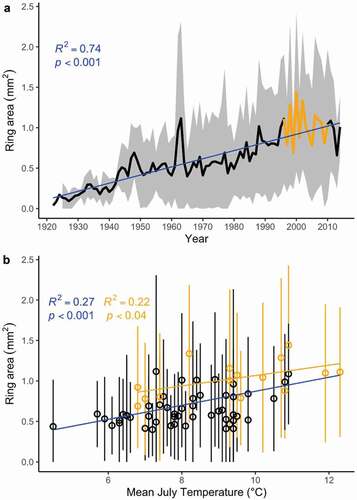
Figure 6. (a) The changes in growth trends and the (b) relationship with July temperature over time. (a) Each point represents the linear model coefficient relating growth and year for the fourteen-year window starting from the year on the x-axis. This linear model was significant if the point is purple. (b) The linear model coefficient for July temperature with ring width or ring area, for the same fourteen-year windows. The results that use data from the same years as our shrub cover analysis correspond to black arrows in each plot