Influence of treatment on rooting of arctic Salix species cuttings for revegetation

Figures & data

Table 1. Experiment 1 model rankings and probabilities for fall and spring cuttings predicting proportion of cuttings that rooted and for cuttings with at least one root, predicting number of roots, longest root length, and proportion with shoot health 5

Fall models rankings	Model probability	Spring models rankings	Model probability
Proportion rooted
Null	0.272	Null	0.393
Soaking	0.234	Concentration	0.168
Concentration	0.111	Soaking	0.152
Concentration + Soaking	0.095	Concentration + Soaking	0.068
Soaking + Soaking^2	0.091	Concentration + Concentration^2	0.068
Concentration + Soaking + Concentration * Soaking	0.071
Concentration + Concentration^2	0.041
Root number
Concentration	0.228	Concentration + Concentration^2 + Soaking + Soaking^2	0.760
Concentration + Concentration^2	0.206	Concentration + Concentration^2 + Soaking	0.218
Concentration + Soaking	0.161	Null	0.000
Concentration + Soaking + Concentration * Soaking	0.138
Concentration + Soaking + Concentration^2	0.113
Concentration + Soaking + Soaking^2	0.093
Null	0.002
Root length
Null	0.276	Concentration + Soaking + Soaking^2	0.568
Soaking	0.205	Concentration + Concentration^2 + Soaking + Soaking^2	0.220
Concentration	0.130	Soaking + Soaking^2	0.140
Soaking + Soaking^2	0.097	Null	0.001
Concentration + Soaking	0.092
Concentration + Concentration^2	0.053
Concentration + Soaking + Concentration * Soaking	0.046
Shoot health of 5
Null	0.404	Null	0.250
Concentration	0.156	Soaking	0.204
Soaking	0.156	Soaking + Soaking^2	0.144
Soaking + Soaking^2	0.070	Concentration	0.096
Concentration + Soaking	0.063	Concentration + Soaking + Concentration * Soaking	0.092
Concentration + Concentration^2	0.060	Concentration + Soaking	0.075

Note. Models were compared using the Akaike information criterion and ranked by weight to determine probability of being the best model for the data. A cumulative probability of at least 0.9 is presented for each dependent variable, along with the null model probability. The evidence ratio (i.e., the relative likelihood of two models, I and j being the best model) can be calculated by dividing the model probability of a higher ranked model by a lower ranked model.

Figure 1. Length of longest primary, secondary, tertiary, and quaternary roots with standard error at day 60 for rooted Salix spp. cuttings in experiments 1 and 2 at different times of year. Length of longest quaternary roots was not assessed for summer cuttings in experiment 1.

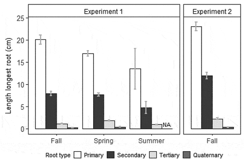
Figure 2. Percentage of fall and spring Salix spp. primary roots with secondary roots per cutting in different secondary root categories (vertical panels) in experiment 1 by IBA concentration (%; x axis) and soaking time (days; horizontal panels) with standard error. All cuttings are present in each secondary root category (vertical panel). Each bar is n = 6 (fall) and n = 9 (spring).

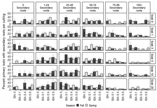
Figure 3. Percentage of fall Salix spp. primary roots with secondary roots per cutting in experiment 2 with secondary roots in different secondary root categories by treatment (x axis) with standard error. All cuttings are present in each root category. Each bar is n = 10 (all rooted cuttings are represented in each secondary root box).

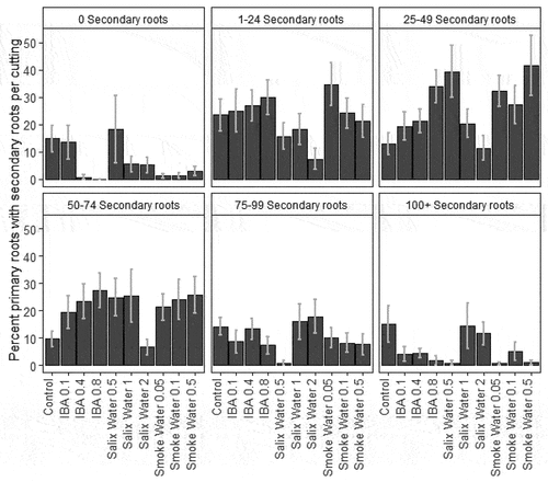
Table 2. Mean difference (Diff) in rooting and percentage change between IBA concentration (0.1, 0.4, 0.8 percent) and control (0 percent) and soaking length (one, three, five, ten, and twenty days) and control (zero days) for number of roots and root length (cm) for Salix cuttings in fall and spring in experiment 1

		Number of roots				Root length (cm)
		Fall		Spring		Fall		Spring
		Diff	% Change	Diff	% Change	Diff	% Change	Diff	% Change
Cuttings with callus
Mean concentration vs. control		4.7	80.3	3.9	41.2	−4.6	−19.2	−2.7	−13
Mean soaking vs. control		−2.6	−21.3	2.3	21.3	−3.8	−15.9	2.6	−15.9
Cuttings without callus
Mean concentration vs. control		0.78	28	2	96.8	9.5	70.4	0.2	4.1
Mean soaking vs. control		−5.2	−83.1	−1.3	−28.5	−7.7	−35.4	−2.9	−44.9
Rooted cuttings
Mean concentration vs. control		3.9	63.1	4.1	46.3	−1.8	−8.6	−2.0	−10.8
	0.1–0	1.5	25.1	2.0	22.3	−1.4	−6.3	−0.7	−3.6
	0.4–0	3.4	55.8	6.1	68.5	−2.1	−9.9	−2.1	−11.3
	0.8–0	6.7	109	4.1	46.6	−2.0	−9.5	−3.2	−17.4
Mean soaking vs. control		−2.5	−22.4	2.2	21.6	−3.3	−14.5	2.5	17.1
	1–0	−2.0	−18.1	−1.2	−11.8	0.5	2.4	−0.4	−2.6
	3–0	−4.4	−39.4	−0.5	−4.9	−5.3	−23.4	1.1	7.2
	5–0	−0.6	−5.3	4.0	39.9	−4.9	−21.7	2.0	13.7
	10–0	−2.9	−26.1	4.9	48.3	−2.0	−8.9	7.1	47.8
	20–0	−2.6	−23.1	3.7	36.5	−4.7	−20.9	2.9	19.4

Figure 4. Number of roots (a) and length longest root (b) with standard error at day 60 for all Salix spp. cuttings in experiment 1 that had callus (solid line) and did not callus (dashed line) by IBA concentration (%; x axis), season (horizontal panels), and soaking time (days; vertical panels).

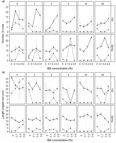
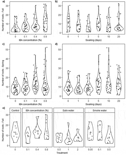
Figure 5. Violin and jitter plots for number of roots in fall (a), (b), (e) and spring (c), (d) on rooted Salix spp. cuttings from experiment 1 for IBA concentration (%) (a), (c); soaking time (days) (b), (d); and from experiment 2 by treatment (e). Closed circles represent individual roots; open circles represent treatment means. Each closed circle in the jitter plot had a small value (between 0 and 0.2) added to the value on the x axis to visually separate points. Black lines for each violin plot use density curves to show data distribution, with wider areas having higher frequency of data points than narrower areas.