Figures & data
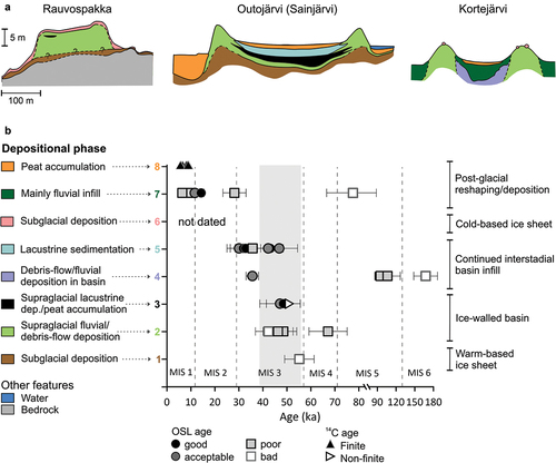
Figure 1. A. Location of map in B and of three interstadial sites mentioned in the text. B. Map showing the distribution of Veiki moraine (in black, from C. Hättestrand Citation1998) and the study area location in the northernmost lobe (the Lainio arc). © EuroGeographics for the administrative boundaries and the CIA World Data Bank II (WDBII) for rivers.
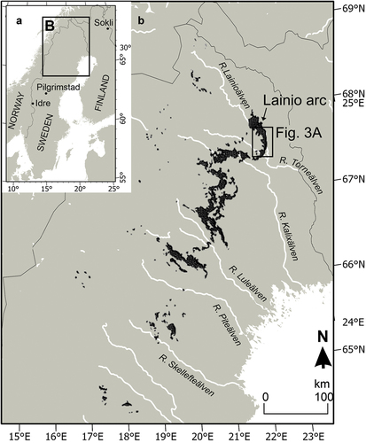
Figure 2. Principle sketch of Veiki moraine formation, modified from Sigfúsdóttir (Citation2013). NB. The profiles are vertically exaggerated. (A) Subglacial thrusting in an active ice sheet brings material to the ice surface and creates a thrust moraine at the margin. (B) As the ice stagnates, debris accumulates on the ice surface and a hummocky landscape develops. (C) Supraglacial sand and diamictons are flowing into basins in the ice where fine-grained lake sediment and organic wetland deposits also formed in some cases. (D) As the ice melts, mass movements bring more material into the basin, covering the lake sediments. (E) The ice melts and the former basin turns into a topographic high (a plateau) in the terrain. (F) The plateau is overridden by cold-based ice, which remolds it slightly and leaves a thin till layer on top.
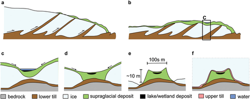
Figure 3. Maps of the field area with details of the four sites. (A) Quaternary deposits map (SGU Citation2014). See for location within Sweden. (B) Hillshade for Rauvospakka. (C) Hillshade for Kortejärvi. (D) Hillshade for Outojärvi and Sainjärvi. Coring locations (K2, O3, S3), trenches (R1, R2), and road cuts (K3) are marked with red dots. Elevation data in (B)–(D) from Lantmäteriet (Citation2015).
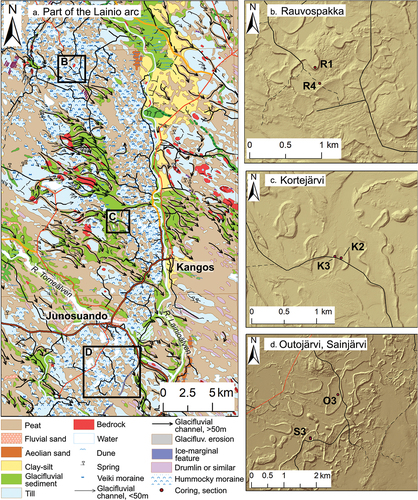
Figure 4. Two Veiki plateaus with different positions in the landscape. (A) The Rauvospakka plateau (photo taken from the south) is relatively high. Sediment infill and peat accumulation occurred at the site during downwasting of an ice sheet; however, after deglaciation the site had no further sediment infill due to its inverted topography (cf. ). (B) Sainjärvi, a plateau at low relative elevation (photo taken from the coring point toward the northwest side of the lake and the forested rim ridge). Due to its position in the landscape this site has acted as a sediment trap both during and subsequent to formation of the Veiki plateau; hence, sediment from the supraglacial formation, the following ice-free period, and the Holocene is expected here (cf. ). The plateaus at Kortejärvi () and Outojärvi () are in this respect similar to Sainjärvi.
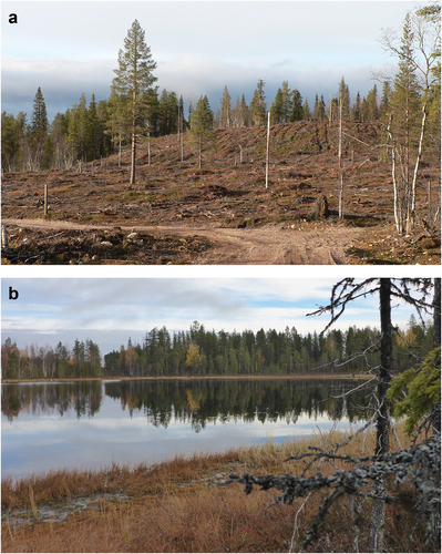
Figure 5. Examples of preheat plateau and dose recovery plots. (A) Sample 12057 from Rauvospakka. Both dose recovery ratio and equivalent dose varies with preheat temperature. Preheat at 220°C (cutheat 200°C) was selected for measurement. (B) Sample 20131 from Outojärvi 3. This sample is more stable but shows relatively large spread and the measured dose tends to underestimate the given dose for lower temperatures. Preheat at 260° (cutheat 220°C) was selected for measurement. Three aliquots per temperature were measured; for sample 20131 all aliquots at 240°C had to be rejected because they failed the acceptance criteria.
Figure 6. Sediment photos. (A) Silty sandy sediments at 2.9 m depth in the Outojärvi core. (B) Gravelly sand at 2.35 to 2.45 cm depth in the Kortejärvi 2 core. (C) Rim ridge sediments at Kortejärvi 3 (Lindqvist Citation2020, site K3A). (D) Peat and sandy–silty laminated sediments overlain by ~3-m diamicton in Rauvospakka trench 1.
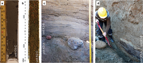
Figure 7. Stratigraphic logs from Outojärvi and Sainjärvi. (A) Outojärvi 3 core. (B) Sainjärvi 3 core. Both mean and modeled OSL ages are shown (most modeled ages are CAM ages, MAM ages are marked with *; ). For further information about the radiocarbon ages, see Table S4. Please note that only the last three digits of the OSL sample number are given here. Ages in gray are considered unreliable based on, for OSL ages, poor luminescence characteristics or incomplete bleaching (poor or bad quality; see Table S2), and for 14C ages, contamination by younger organic material that was pushed down during coring; see further explanation in text.
Figure 8. Stratigraphic logs. (A) Kortejärvi 2 core. Redrawn from Lindqvist (Citation2020). (B) Composite log from road cuts at Kortejärvi 3 (based mainly on K3A). Samples marked with # are taken from the same unit but in other exposures; see Table S2 or details in Lindqvist (Citation2020). Redrawn from Lindqvist (Citation2020). (C) Composite log from Rauvospakka trench 1. Drawn after Sigfúsdóttir (Citation2013). (D) Composite log from Rauvospakka trench 4. Drawn after Sigfúsdóttir (Citation2013). For legend, see . Both mean and modeled OSL ages are shown (most modeled ages are CAM ages; MAM ages are marked with *; ). For further information about the radiocarbon ages, see Table S4. Please note that only the last three digits of the OSL sample number are given here. Ages in gray are considered unreliable based on, for OSL ages, poor luminescence characteristics or incomplete bleaching (poor or bad quality, see Table S2) and, for 14C ages, contamination by younger organic material that was pushed down during coring; see further explanation in text.
Table 1. Lithofacies associations at the four sites. See for legend.
Figure 9. Examples of decay and growth curves. (A) Sample 20129 from Outojärvi 3 has a relatively strong signal dominated by a fast component (fast ratio FR = 31 for this aliquot) that contributes 68 percent of the initial signal. The signal continues to grow to high doses. (B) Sample 20138 from Sainjärvi 3 has a dim signal that has a weaker fast component (53 percent of the initial signal, FR = 6). Both samples have a relatively high background (slow signal component).
Table 2. Sample information and luminescence data, sorted by lab number (this is also in stratigraphic order for all sites but Kortejärvi 3, which is a composite site). See for context and Table S2 for additional luminescence data; for example, overdispersion values and basis for age reliability assessment.
Figure 10. Dose distributions shown as probability plots. (A) Sample 20139 from Sainjärvi 3 has a broad but not significantly skewed dose distribution. (B) Sample 19007 from Kortejärvi 2 has a significantly positively skewed dose distribution. Note that aliquots that lack error bars are those for which Analyst software could not calculate an error due to the dose being at or close to saturation. Both samples were measured as 4-mm aliquots.
Figure 11. (A) Schematic cross-profiles of the studied Veiki moraine plateaus with interpreted sediment architecture. See (B) for legend. The profiles from Rauvospakka and Kortejärvi are based on information from ground penetrating radar, trenches, and coring (Sigfúsdóttir Citation2013; Lindqvist Citation2020), whereas the profile from Outojärvi, which is also taken to represent Sainjärvi, is modified from a coring-based profile in Lagerbäck (Citation1988b). The profiles are vertically exaggerated and thin units have been made larger for visibility. (B) OSL mean ages and 14C ages from the four sites separated into groups based on stratigraphic, sedimentological, and geomorphological context and related to different depositional phases in the Veiki moraine formation and subsequent development (see text for explanation). The gray shading indicates our best estimate of the time of formation as ice-walled basins, 56 to 39 ka. Due to low-precision ages the age span is wide but clearly in MIS 3, not MIS 5c. Ages classified as poor or bad are considered unreliable due to methodological issues; see text and Table S2 for details.