Figures & data
Figure 1. Location of the OSL data observation points based on published data before 2020 in Finland (see Supplementary data), in the central part of Last Glacial Maximum. Modified from Sarajärvi (Citation2020).
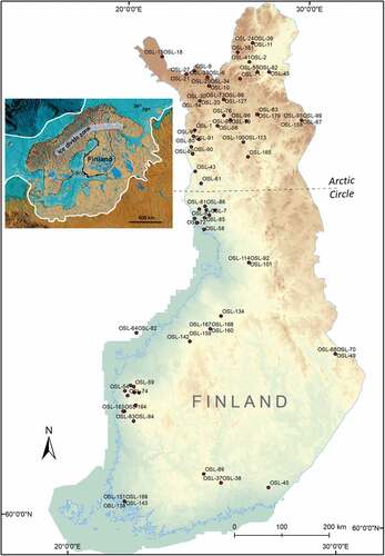
Figure 2. A plot of between-cluster sum of squares divided by the total sum of squares (BSS/TSS ratios) for different values of K. The “elbow” is marked by the green circle. The “right” number of clusters as indicated by the plot is six to eight.
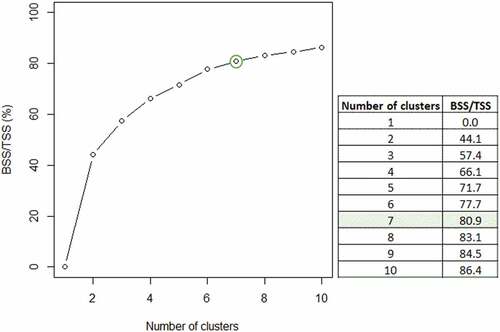
Figure 3. The K-means algorithm applied to the OSL data results in an optimal number of clusters of seven. This seven-cluster solution is shown in the scatterplot matrix, where all variable pairs (age [ka], age standard error [ka], dose rate [Gy/ka], and paleodose [Gy]) are shown against each other, in their original units. The colors for the observations are according to the cluster assignments to the seven clusters.
![Figure 3. The K-means algorithm applied to the OSL data results in an optimal number of clusters of seven. This seven-cluster solution is shown in the scatterplot matrix, where all variable pairs (age [ka], age standard error [ka], dose rate [Gy/ka], and paleodose [Gy]) are shown against each other, in their original units. The colors for the observations are according to the cluster assignments to the seven clusters.](/cms/asset/8a1a5c7f-1a5b-45f2-9c74-7510b51147b5/uaar_a_2117765_f0003_oc.jpg)
Table 1. Basic parameters of the seven clusters formed after using function kmeans().
Figure 4. The model-based cluster algorithm using the function mclust() results in an optimal model with K = 5 clusters and visualizes the estimated cluster centers and shapes (ellipses). This five-cluster solution is shown in the scatterplot matrix with the scales in the original units (age [ka], age standard error [ka], dose rate [Gy/ka], and paleodose [Gy]) and with different colors of the observations as they are assigned to the clusters; the ellipses indicate the cluster shapes.
![Figure 4. The model-based cluster algorithm using the function mclust() results in an optimal model with K = 5 clusters and visualizes the estimated cluster centers and shapes (ellipses). This five-cluster solution is shown in the scatterplot matrix with the scales in the original units (age [ka], age standard error [ka], dose rate [Gy/ka], and paleodose [Gy]) and with different colors of the observations as they are assigned to the clusters; the ellipses indicate the cluster shapes.](/cms/asset/37d95923-788c-4493-b0af-e6b8c7cd6840/uaar_a_2117765_f0004_oc.jpg)
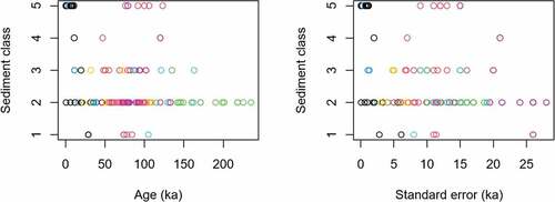
Figure 5. Distribution of different sediment classes in relation to the seven clusters defined by the function kmeans(). Sediment classes are as follows: Class 1 = glaciolacustrine/lacustrine deltaic fine sand/silt, Class 2 = glaciofluvial/-lacustrine or fluvial/lacustrine stratified sand, Class 3 = glaciofluvial medium/coarser sand sediments, Class 4 = lacustrine or glaciolacustrine littoral deposits with gravel and sand matrix, Class 5 = ice-wedge cast sand infills and eolian dune sediments. See cluster classification in .