Plant succession on glacial moraines in the Arctic Brooks Range along a >125,000-year glacial chronosequence/toposequence

Figures & data

Figure 1. Study site locations. From youngest to oldest, the Grizzly Glacier site includes ELIA and NEO, Itkillik II aged glacial deposits are located at ITKII-AP and near the toe of Slope Mountain in the foothills (ITKII-N), and ITKI and SAG are located between Imnavait Creek and Toolik Lake in the foothills. Map created by Dr. Martha Raynolds at the University of Alaska Fairbanks.

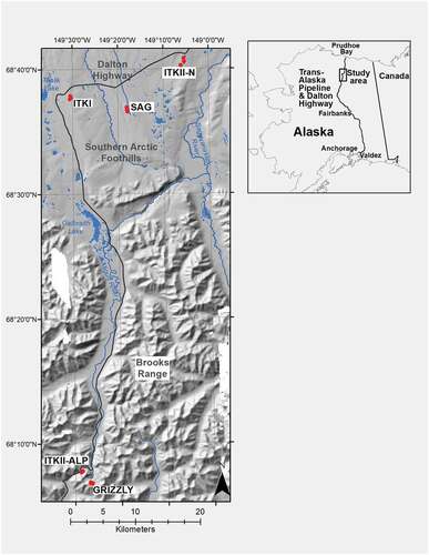
Table 1. Study site characteristics and plots sampled per site.

Glacial deposit	Average elevation (M)	Latitude and longitude (DD)	Estimated age (years BP)	Rock relevés (N)	Fine-grained relevés (N)
ELIA	1,700	68.1133 N, 149.4426 W	22–36	3	3
NEO	1,700	68.1132 N, 149.4386 W	238–500	3	3
ITKII-AP	1,500	68.1299 N, 149.4770 W	10,000–15,000	4	4
ITKII-N	800	68.6762 N, 149.0888 W	10,000–15,000	5	5
ITKI	900	68.8672 N, 149.5101 W	25,000–75,000	3	3
SAG	950	68.6125 N, 149.30016 W	125,000–150,000	3	3
(N plots = 42)	Δaltitude = 900 m		$\mathrm{\Delta }\mathit{time}=\ge$124,978 years	N = 21	N = 21

Figure 2. (Top) Grizzly Glacier cirque photographed and used with permission by Jim Ellis in July 1977. (Bottom) The same general scene photographed by SK (formerly S. Gowan) in July 2017. These photographs were taken from slightly different locations and distances from the glacier. Red arrows indicate moraine features for comparison of ice mass.

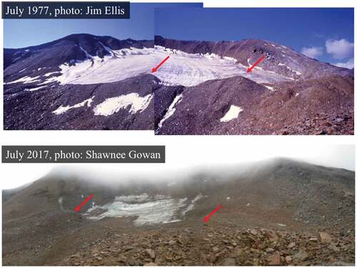
Figure 3. Examples of (A) rock and (B) fine-grained substrate plots on each glacial deposit surface in order of the estimated age since deglaciation.

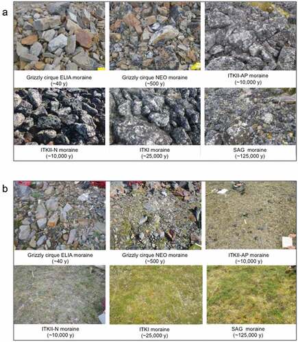
Figure 4. Five maximum thallus radius measurements taken across both the ELIA (triangles) and NEO (squares) moraines in the Grizzly Glacier cirque from three different lichen taxa: Rhizocarpon geographicum s.l. (shown in black) and Pseudephebe spp. and Umbilicaria spp. (shown in gray). Age estimates were derived from growth rates presented in (Calkin and Ellis 1980). Red symbols represent average age estimates of the five largest thalli on both moraines.

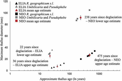
Figure 5. Cluster analysis of plots (n =42) from 1,700 to 800 m.a.s.l. and from 22 to 125,000 years since deglaciation in the central Brooks Range, north into the Arctic foothills. Study plot numbers are along the left axis (red = rocky plots; green = fine-grained plots). Seven main clusters of plots are defined by large red numbers. Groups with highest percentage floristic similarity are located closest to the left edge of the diagram; dissimilarity increases as subgroup nodes expand away from branch tips. Scale bar (top) shows percentage similarity for each cluster.

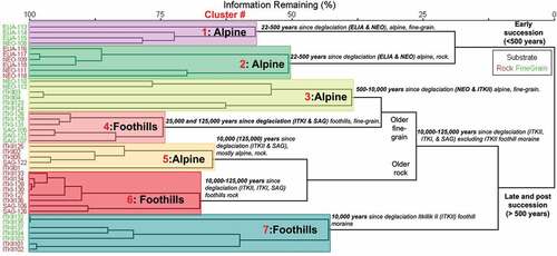
Figure 6. Timeline of major changes to vegetation communities on both (A) fine-grained and (B) rock substrates across a 125,000 year chronosequence and 900 m altitudinal gradient.

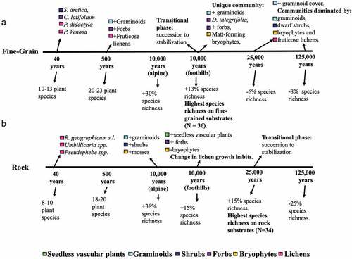
Table 2. Plant community type summary table with characteristic species for each community type defined across the sequence.

Community type name	Community type age	Community type elevation and substrate	Characteristic species
Cluster 1: Chamerion latifolium and Peltigera didactyla	40–500 years (ELIA and NEO)	≥1,700 m.a.s.l., fine-grained	Foliose lichens Peltigera didactyla and Peltigera venosa, erect forb Chamerion latifolium, and dwarf shrub Salix arctica
Cluster 2: Lecanora polytropa and Candellariella vitellina	40–500 years (ELIA and NEO)	≥1,700 m.a.s.l, rock	Crustose lichens Candellariella vitellina and Lecanora polytropa and foliose lichen Umbilicaria cylindrica
Cluster 3: Salix rotundifolia and Racomitrium lanuginosum	500–10,000 years (NEO and ITKII-AP)	≥1,700 m.a.s.l., fine-grained	Fruticose lichen Dactylina ramulosa; rush Luzula confusa; erect forbs Draba macrocarpa, Saxifraga cernua, and Saxifraga razshivinii; and dwarf shrub Salix rotundifolia
Cluster 4: Betula nana and Masonhalea richardsonii	25,000–125,000 years (ITKI and SAG)	900–950 m.a.s.l., fine-grained	Fruticose lichens Cladonia bellidiflora and Cladonia sulphurina; foliose lichens Masonhalea richardsonii, Peltigera canina, and Sticta arctica; cushion forb Diapensia lapponica; erect forb Polygonum bistorta; grass Poa alpina; low shrubs Cassiope tetragona and Vaccinium vitis-idaea; and dwarf shrub Betula nana
Cluster 5: Porpidia flavocaerulescens and Cladonia squamosa	10,000 years (ITKII-AP)	1,400 m.a.s.l., rock	Crustose lichen Porpidia flavocaerulescens and Schaereria endocyanea, fruticose lichen Cladonia squamosa, foliose lichens Cetraria nigricans and Umbilicaria torrefecta, and mosses Schistidium apocarpum and Tortella tortuosa
Cluster 6: Arctoparmelia centrifuga and Ophioparma lapponicum	10,000–125,000 (ITKII-N, ITKI, SAG)	800–950 m.a.s.l., rock	Crustose lichens Ophioparma lapponica and Rhizocarpon cinereovirens and foliose lichen Arctoparmelia centrifuga and Asahinea scholanderi
Cluster 7: Mixed plant community cluster	25,000 years (ITKII-N)	800 m.a.s.l., fine-grained	Crustose lichen Ochrolechia upsaliensis; foliose lichens Hypogymnia austerodes and Lobaria linita; moss Tomenthypnum nitens; mat forb Dryas integrifolia; erect forbs Antennaria friesiana, Bistorta vivipara, Oxytropis jordalii, Pedicularis lanata; and sedge Kobresia myosuroides

‘

Figure 7. (A), (B) Average species richness and (C), (D) total percentage cover of major growth forms on (A), (C) fine-grained and (B), (D) rock substrates across chrono- and toposequences (ELIA =26–40 years since deglaciation, NEO =238–475 years since deglaciation, ITKII =10,000–25,000 years since deglaciation, ITKI =25,000–75,000 years since deglaciation, and SAG =125,000–780,000 years since deglaciation).

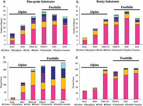
Table 3. Percentage change and number of plant species accumulated or lost from one glacial surface to the next across the chronosequence.

	ELIA to NEO (22–500 years) change in species richness		NEO to ITKII-AP (500–10,000 years) change in species richness		ITKII-AP to ITKII-N (10,000 years) change in species richness		ITKII-N to ITKI (10,000–25,000 years) change in species richness		ITKI to SAG (125,000+ years) change in species richness
	Alpine		Alpine		Alpine to foothills		Foothills		Foothills
	Species percentage change	Species added or lost	Species percentage change	Species added or lost	Species percentage change	Species added or lost	Species percentage change	Species added or lost	Species percentage change	Species added or lost
Rock	56	+10	38	+11	15	+5	15	+6	−25	−10
Fine-grained	44	+10	30	+10	13	+5	−6	−2	−8	−3

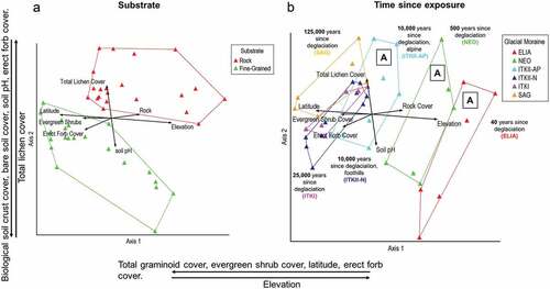
Figure 8. NMS ordination grouped by (A) substrate and (B) time since exposure. Bi-plots (represented by arrows) within ordinations represent environmental factors with a Pearson’s correlation coefficient $r^2\ge 0.3$. Axes are labeled with variables having strong Kendall’s tau ($\mathit{\tau }>0.3)$ correlation coefficients. Groups marked “A” in (B) indicate alpine glacial deposits.

Calkin, P. E., and J. M. Ellis. 1980. A lichenometric dating curve and its application to Holocene glacier studies in the central Brooks Range, Alaska. Arctic and Alpine Research 12 (3):245. doi:10.2307/1550713.

 Web of Science ®Google Scholar