Figures & data
Figure 1. Location map showing (a) the location of the study area on the Greenland Ice Sheet and (b) the location of Nunatakassaap Sermia (NS) and Illullip Sermia (IS). Black lines show transects used to sample ice velocity data. Blue lines show transect used to sample surface elevation change and to calculate excess buoyancy. Image source: Landsat 8, USGS Earth Explorer, 10 August 2020. Landsat imagery is overlain with ice velocities for winter 2017–2018. Source: Joughin et al. (Citation2010, Citation2015, updated 2018).
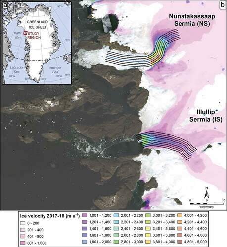
Figure 2. Frontal position relative to 9 April 1976 for (a), (b) Nunatakassaap Sermia (NS) and (c), (d) Illullip Sermia (IS). Terminus positions are color-coded according to date for (a) NS and (c) IS. NS’s terminus has remained attached to the pinning point at its northern margin (Point I, (a)). Gray boxes indicate the reference box used to calculate relative frontal positions. Base image source: Landsat 8, USGS Earth Explorer, 10 August 2020. Frontal positions are plotted over time and relative to 20 July 1976 for (b) NS and (d) IS. Note the differing y-axis scales for (b) and (d).
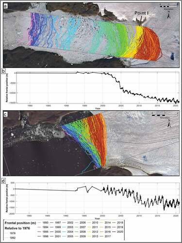
Figure 3. Interannual winter velocity changes at (a) Nunatakassaap Sermia (NS) and (b) Illullip Sermia (IS). Ice velocities are color-coded according to year of the winter velocity mosaic. Note that NS had a floating ice tongue in 2000–2001, which had collapsed by the subsequent winter velocity mosaic in 2005–2006. X-axis values are relative to the 2000–2001 termini for each glacier. Source: Joughin et al. (Citation2010, Citation2015, updated 2018).
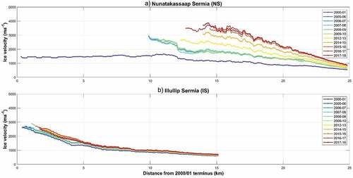
Figure 4. Seasonal variations in ice velocities at Nunatakassaap Sermia (NS) for (a) spring, (b) summer, (c) autumn, and (d) winter. Ice velocities are color-coded according to date. X-axis values are relative to the 2000–2001 termini for each glacier. Source: Joughin et al. (Citation2020; seasonal velocity data from 2009 to 2018).
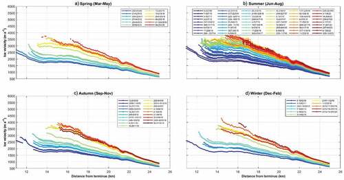
Figure 5. Seasonal variations in ice velocities at Illullip Sermia (IS) for (a) spring, (b) summer, (c) autumn, and (d) winter. Ice velocities are color-coded according to date. X-axis values are relative to the 2000–2001 termini for each glacier. Source: Joughin et al. (Citation2020; seasonal velocity data from 2009 to 2018).
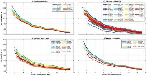
Figure 6. Seasonal velocity cycles between 2009 and 2020 for (a) Nunatakassaap Sermia (NS) and (b) Illullip Sermia (IS). For each glacier, data were sampled at the most retreated 2020 terminus and then at 1-km intervals inland for six intervals. This enabled the spatial pattern of seasonal velocity to be determined but accounted for terminus retreat. Velocity data are color-coded by distance inland and frontal position relative to 9 April 1976 is shown in black.
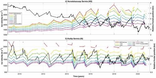
Figure 7. (a) Surface elevation changes at Nunatakassaap Sermia (NS) between 2010 and 2017. Elevation profiles are color-coded by year, and each year is composed of multiple profiles. Surface elevation data were extracted from Arctic digital elevation model (DEM) tiles along the glacier centreline and the x-axis distance is relative to the 2000–2001 glacier termini in the Joughin et al. (Citation2010, Citation2015, updated 2018). (b) Excess buoyancy, calculated at the same sample points as in (a), using Arctic DEM tiles and bed topography from BedMachine v3 (black line). Transcripts are color-coded by date. Red line indicates where Hb equals 50 m, below which previous work suggests that calving rates will increase (Meier et al. Citation1994).
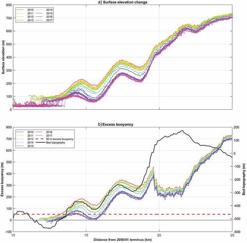
Figure 8. (a) Surface elevation changes at Illullip Sermia (IS) between 2010 and 2017. Elevation profiles are color-coded by year, and each year is composed of multiple profiles. Surface elevation data were extracted from Arctic digital elevation model (DEM) tiles along the glacier centreline and the x-axis distance is relative to the 2000–2001 glacier termini in the Joughin et al. (Citation2010, Citation2015, updated 2018). (b) Excess buoyancy, calculated at the same sample points as in (a), using Arctic DEM tiles and bed topography from BedMachine v3 (black line). Transcripts are color-coded by date. Red line indicates where Hb equals 50 m, below which previous work suggests that calving rates will increase (Meier and Reeh Citation1994).
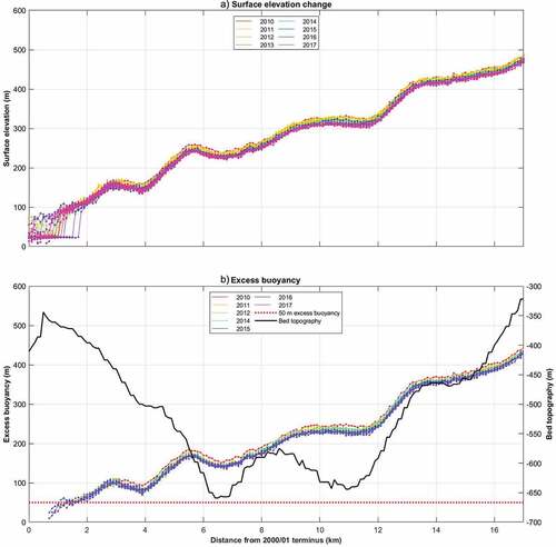
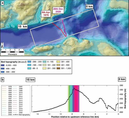
Figure 9. Basal topography of Nunatakassaap Sermia (NS). (a) Topography beneath NS and within its fjord, determined from BedMachine v3 (Morlighem et al. Citation2017). Contour interval is 200 m. White box indicates the extent of the reference box used to digitize terminus positions, and the terminus locations are marked for the earliest (9 April 1976; red) and latest (26 December 2020; pink) frontal positions available during the study period. (b) Location of NS’s terminus through time, relative to the upstream end of the reference box. Frontal positions are color-coded by year. Bed topography (black line) along the center of the reference box.

Figure 10. Calving rates and their relationship with potential controls for Nunatakassaap Sermia (NS) (left-hand panels) and Illullip Sermia (IS) (right-hand panels). Calving rates in meters per day (m d−1) for (a) NS and (b) IS. Positive values indicate a net loss of ice via calving for a given time period (i.e., the rate of frontal retreat exceeds the forward ice velocity) and negative values indicate a net gain (i.e., the rate of frontal retreat is less than the forward ice velocity). Zero calving rate indicates that the rate of frontal retreat exactly balances the forward ice velocity. (c), (d) Relative frontal position (kilometers, relative to 9 April 1976) and terminus ice velocities in meters per day, to provide context for the calving rates. Calving rate regressed against mean ice thickness across the terminus at the time the calving rate was calculated, for (e) NS and (f) IS. The regression line is plotted in black and the R2 and p values for the regression are displayed above the plot. (g), (h) Same as (e) and (f) but for mean water depth at the terminus.
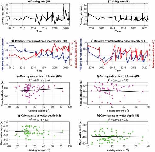
Figure 11. Basal topography of Illullip Sermia (IS). (a) Topography beneath IS and within its fjord, determined from BedMachine v3 (Morlighem et al. Citation2017). Contour interval is 100 m. White box indicates the extent of the reference box used to digitize terminus positions, and the terminus locations are marked for the earliest (9 April 1976; red) and latest (22 September 2018; pink) frontal positions available during the study period. (b) Location of IS’s terminus through time, relative to the upstream end of the reference box. Frontal positions are color-coded by year. Bed topography (black line) along the center of the reference box.