Figures & data
Figure 1. Study area map within the Copper River Basin of Southcentral Alaska showing Copper River and tributaries, study reaches, nearby communities, roads, boundaries of Wrangell–St. Elias National Park and Preserve, and Alaska Native Corporation lands within those boundaries. Land status from Bureau of Land Management and Alaska Department of Natural Resources and topography from Esri, FAO, NOAA, USGS.
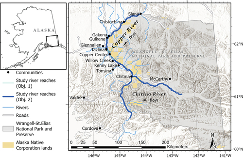
Figure 2. Example of low (left panel) and high (right panel) ice extent classes shown for segments of the Copper River study reach north of Copper Center. Classes were assigned by interpreting Landsat images at 60-m resolution to be consistent across sensors. Landsat 8 images are shown in the resampled 60-m resolution and original 30-m resolution and are displayed as RGB composites with SWIR, NIR, and green bands. Below are photographs taken from a fixed time-lapse camera (left; Bondurant et al. Citation2022) and citizen science observer (right; Fresh Eyes on Ice Citation2022) on the same dates as the satellite image acquisitions. Open water is present in both low and high ice extents. Red arrows indicate the location of open water pictured in the photographs on the Landsat images.
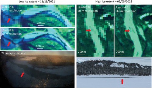
Table 1. Characteristics of ice extent classes for a 30-km segment of the Copper River by Copper Center, as interpreted from Landsat imagery.
Figure 3. Landsat data used in the analysis of historic ice phenology summarized by month and year. Cell values represent the number of unique image dates. Multiple scenes from the same image date were mosaicked together. Color scale ranges from white to green representing relatively low to high values.
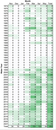
Figure 4. Examples of Sentinel-1 SAR image processing: (a) Sentinel-2 optical reference image (true color); (b) SAR single-date image (VV backscatter); (c) SAR multitemporal composite (red: VV backscatter from autumn, green: VV backscatter from 26 January 2021, blue: VV backscatter from autumn); (d) SAR classification of water and ice for single-date using a threshold on VV, overlain on SAR multitemporal composite; (e)–(g) SAR seasonal composites of classified images showing water occurrence from November to February for WYs 2018, 2019, and 2020, overlain on optical image (Sentinel-2, 26 January 2021); and (h) SAR multiyear composite showing water occurrence from November to February averaged for WYs 2018 to 2020, overlain on optical image (Sentinel-2, 26 January 2021).
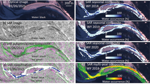
Figure 5. Sentinel-1 SAR classification of water and ice. A threshold of VV backscatter intensity (dB) was determined through histogram analysis of training pixels (a), and an accuracy assessment was conducted with a validation data set (b). Confusion matrix (b) shows predicted versus actual classes, with count of validation pixels in bold.
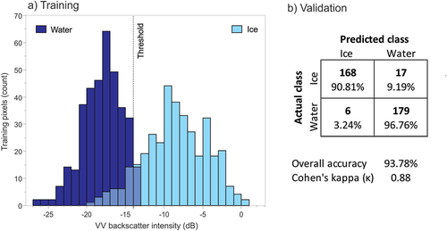
Table 2. Summary of Sentinel-1 SAR scenes used for analysis of river freeze-up and open water persistence for each WY by satellite.
Figure 6. Matrix of gap-filled ice extent observations derived from Landsat imagery for the 30-km study reach of the Copper River near Copper Center, summarized by week and water year.
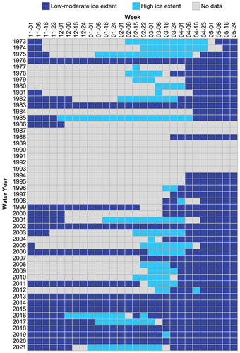
Figure 7. Weekly occurrence of high ice extent expressed as percentage of total Landsat-derived observations by time period (WYs 1973–1997 and WYs 1998–2021) for the Copper River study reach, showing the reduced occurrence of high ice extents in the recent time period. The majority of weekly observations by time period were of high ice extents for the points above the dashed reference line (>50 percent). Statistical significance of weekly contingency analyses conducted from 8 February through 8 April is denoted as *p < .1 and **p < .05.
Figure 8. Change over time in the probability of high ice extents on Copper River study reach from logistic regression analyses of Landsat-derived observations. (a) Weekly probability curves over the full time series (WYs 1973–2021) and (b) comparison of probability between the first and last years of the time series (WYs 1973 and 2021). Decreasing trends in probability of high ice extents were found for all weeks tested. Statistical significance was denoted as *p < .1, **p < .05, ***p < .01.
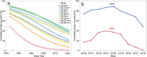
Table 3. Logistic regression models for log odds of high ice extent (derived from Landsat imagery) for Copper River (30-km study reach by Copper Center) by WY (1973–2021) for each week from late winter (8 February) to spring (8 April).
Figure 9. Statistical significance of relationships between weekly Copper River ice extent and climate indices (AFDD and thirty-one-day prior mean air temperature). LogWorth (−log(p value)) is shown as a measure of statistical significance for ease of visualization, with dotted reference lines indicating equivalent p values. Weekly ice extent was significantly related to AFDD throughout this time period and with thirty-one-day prior mean air temperature during March and early April.
Figure 10. Trend and variation in AFDDOct-Apr anomaly from WYs 1943 to 2021, derived from local daily mean air temperatures. Positive anomalies (colder than average) are shown with blue bars and negative anomalies (warmer than average) are shown in red. Statistics for simple linear regression are reported with the 95 percent confidence interval for the mean response shown in gray, indicating a 15% decline in AFDDOct-Apr and a long-term warming trend.
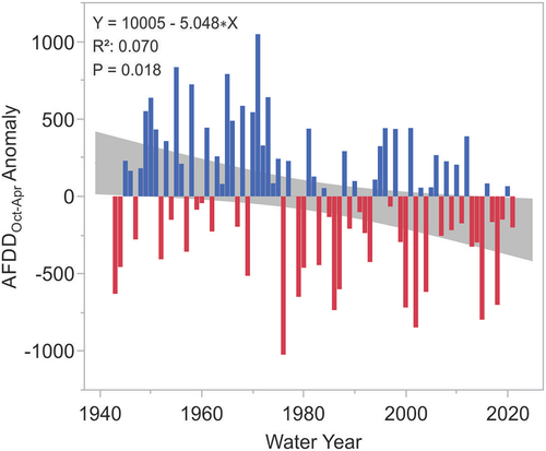
Figure 11. Geospatial patterns of late-winter open water area (top panel) and hydrologic characteristics (bottom panel) of Copper and Chitina rivers by 5-km reach. Numbers along the Copper River indicate river-km at tributaries that demarcate reaches with distinct hydrologic characteristics referenced in . Total areas of open water in late winter were calculated from Sentinel-2 multispectral images acquired in the WY on dates indicated. Hydrologic characteristics include river slope, flow accumulation, cumulative channel width, and unit stream power. Flow direction is indicated by arrows, and nearby communities are shown. Study reaches with no data are depicted in gray.
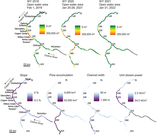
Figure 12. Profile of late-winter open water area and hydrologic characteristics of the Copper River by 5-km subreach. Solid vertical lines indicate locations of tributaries used to demarcate reaches with distinct characteristics. Names of these tributaries are shown in bold italics. Dotted vertical line shows the location of a canyon that influences hydrology. The locations of nearby communities are indicated with normal text. Open water areas were derived from Sentinel-2 imagery from late January/early February in the WYs indicated.
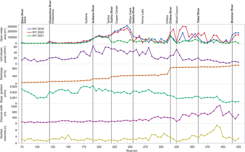
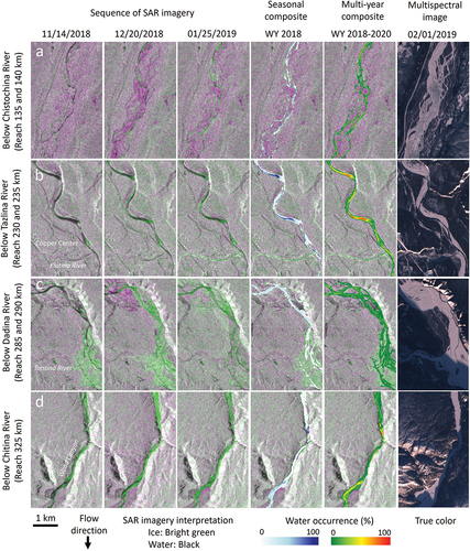
Figure 13. Examples of the freeze-up progression and open water occurrence along distinct stretches of the Copper River with Sentinel-1 SAR imagery and Sentinel-2 multispectral imagery (European Space Agency). The sequence of SAR imagery from three winter dates in WY 2018 are composites that include an autumn scene (open water prior to freeze-up) and a winter scene (red: VV autumn, green: VV winter, blue: VV autumn) and were used to optimize visualization of open water (black) and ice cover (bright green). The seasonal composite is a classified SAR product showing pixel-based water occurrence as a percentage of scenes for the season November to February in WY 2018, overlain on a SAR image. The multiyear composite shows the average water occurrence for November to February over three years (WYs 2018, 2019, 2020) to identify places that tend to remain open late in the winter year after year. The multispectral image (Sentinel-2) was used to calculate late-winter open water area and validate SAR imagery and products.