Drivers of winter ice formation on Arctic water bodies in the Lena Delta, Siberia

Figures & data

Figure 1. Overview of the study site with (a) the location of the two islands in the southern central part of the Lena River Delta. (b) The investigated lakes on Samoylov Island and coring site of the Lena River opposite the Samoylov research station. (c) The investigated lakes on Kurungnakh Island (Höfle 2015; Landsat imagery).

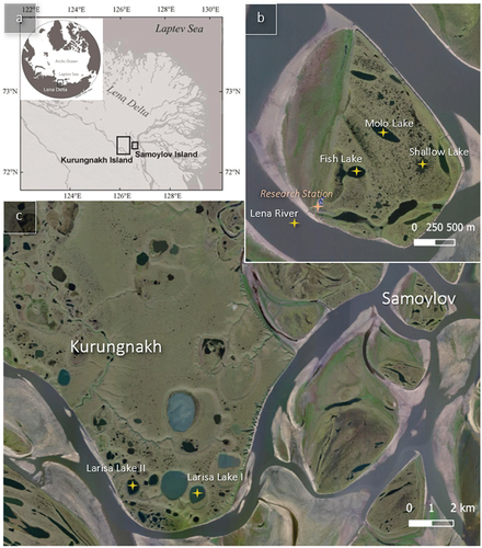
Table 1. List and aerial image of the investigated water bodies and the retrieved ice cores, their coring depths, and the coordinates.

					Coordinates
Water body		Site	Core	Core depth (m)	LAT	LON
	Shallow Lake	SAM	LD16-BH-6 LD18-BH-3 LD18-BH-9	2.32 2.01 1.63	n/a N72.375169 N72.375011	n/a E126.511306 E126.510853
	Molo Lake	SAM	LD18-BH-4	1.81	N72.377942	E126.497124
	Larisa Lake I	KUR	LD18-BH-12	2.00	N72.295004	E126.204703
	Larisa Lake II	KUR	LD18-BH-11	1.83	N72.297046	E126.118249
	Fish Lake	SAM	LD18-BH-6	1.50	N72.373781	E126.487333
	Lena River	OLE	LD13-BH-1 LD18-BH-8 LD19-BH-2	1.65 1.46 1.76	N72.367764 N72.367545 n/a	E126.467666 E126.468242 n/a

Table 2. List of the investigated water bodies and their morphometric characteristics relevant for freezing.

Water body	Deposit type	Area (km^2)	Volume (m^3)	Depth average/max (m)	Geomorphological water body type	Freezing system
Shallow Lake	HOL	0.026^a	18 800^b	1.0/3.1^a	Polygonal/thermokarst lake	Closed
Molo Lake	HOL	0.042^a	103 600^b	2.6/6.2^a	Thermokarst lake	Closed
Larisa Lake I	PLE	0.421^c	n/d	8.1^c	Thermokarst lake	Closed
Larisa Lake II	PLE	0.323^c	n/d	$\sim$8	Thermokarst lake	Closed
Fish Lake	HOL	0.049^a	106 500^b	3.8/12.7^a	Thermokarst lake	Open?
Lena River	n/a	n/a	n/a	$\sim$25	River	Open

Note. The deposit types refer to the elevated Holocene terrace (HOL) in the east of Samoylov Island and the remnant of a Pleistocene accumulation plain (PLE) on Kurungnakh Island where the investigated lakes are located. The river channels have not been assigned to certain deposit types. We assumed Larisa Lake II to be similar in depth to Larisa Lake I, due to both their similar location and morphometric characteristics.

Sources. ^aChetverova et al. (2017). ^bBoike et al. (2015). ^cMorgenstern, Grosse et al. (2011) and Morgenstern, Röhr et al. (2011).

Table 3. Characterization of the four winters during which the investigated ice cores grew.

Water body	Core	Core depth (m)	Freeze-up date (est.)	Coring date	FDD	Snow depth on core (m)	Snow depth SAM (m)
Shallow Lake	LD16-BH-6	2.32	1 October 2015	19 April 2016	4,709	0	0.22
	LD18-BH-3	2.01	2 October 2017	24 April 2018	4,864	0	0.25
	LD18-BH-9	1.63	2 October 2017	6 May 2018	4,976	0.25	0.28
Molo Lake	LD18-BH-4	1.81	2 October 2015	24 April 2016	4,864	0	0.25
Larisa Lake I	LD18-BH-12	2.00	2 October 2017	7 May 2018	4,988	0.1	0.28
Larisa Lake II	LD18-BH-11	1.83	2 October 2017	7 May 2018	4,988	0.1	0.28
Fish Lake	LD18-BH-6	1.50	2 October 2017	29 April 2018	4,917	0.4	0.31
Lena River	LD13-BH-1	1.65	19 October 2012	20 April 2013	5,160	0.42	0.86
	LD18-BH-8	1.46	19 October 2017	4 May 2018	4,955	0.36	0.28
	LD19-BH-2	1.76	19 October 2018	10 April 2019	4,071	0.2	0.18

Note. “Core depth” is the maximum ice thickness at the time of coring; “FDD” is the freezing-degree days calculated from the estimated day of freeze-up until the day of coring; “Snow cover on core” was observed at the time of coring and “Snow depth at SAM” is from the meteorological station.

Figure 2. Characterization of the four investigated ice-growing periods 2012–13, 2015–16, 2017–18 and 2018–19 by (a) snow depth and (b) air temperature (calculated by average values for each day). Meteorological data were provided by the Samoylov long-term observatory (Boike et al. 2019b).

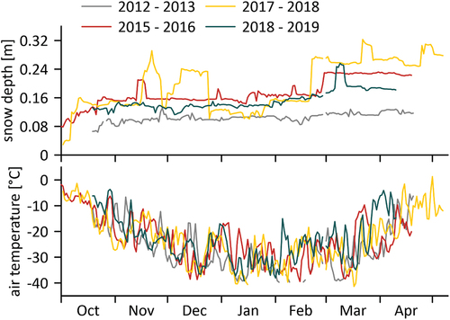
Table 4. Snow depth and air temperature data for the four ice-growing periods (estimated freeze-up until coring), provided by the Samoylov long-term observatory.

Winter	Snow depth (m)			Air temperature (°C)
	Minimum	Average	Maximum	Minimum	Average	Maximum
2012–2013	0.06	0.11	0.13	−39.7	−27.4	−5.5
2015–2016	0.08	0.17	0.23	−39.9	−23.3	−1.8
2017–2018	0.1	0.19	0.32	−43.7	−24.4	1.3
2018–2019	0.11	0.15	0.26	−39.9	−23.4	−3.7

Figure 3. Ice morphology, stable isotope signatures, EC, and modeled ice growth (for selected cores) for group I ice cores.

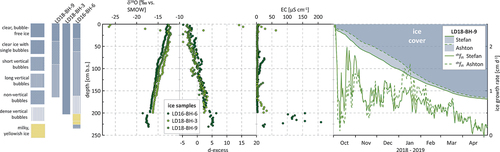
Figure 4. Ice morphology, stable isotope signatures, EC, and modeled ice growth (for selected cores) for group II ice cores.

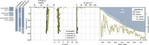
Figure 5. Ice morphology, stable isotope signatures, EC, and modeled ice growth (for selected cores) for group III ice cores.

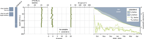
Figure 6. Ice morphology, stable isotope signatures, EC, and modeled ice growth (for selected cores) for group IV ice cores.

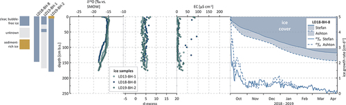
Table 5. Typical values of α, the fitting parameter for calculation of ice thickness using Stefan (Equation (2))(2) $h_i=\mathit{\alpha }\sqrt{\mathit{FDD}}$(2) .

Ice cover condition	α^a
Windy lake, no snow	2.7
Average lake with snow	1.7–2.4
Average river with snow	1.4–1.7
Sheltered small river	0.7–1.4

Note. ^aWith FDD calculated using degrees Celsius and ice thickness in centimeters.

Source. After Michel (1971).

Table 6. Calculated Ashton ice thicknesses vary based on chosen input parameters.

Symbol	Description	Value
ρi	Ice density	917 kg/m^3
Lf	Latent heat of fusion	3.36 × 10^5 J/kg
Tm	Freezing temperature of water	0°C
ki	Thermal conductivity of ice	2.24 W/m°C
Has	Heat transfer coefficient, snow–air interface	20 W/m^2
Hwi	Heat transfer coefficient, ice–water interface	864.6 W/m^2°C
ks → ρs	Snow density
	Freshly fallen snow	0.08–0.16 g/cm^3a
	Damp new snow	0.1–0.2 g/cm^3b
	Settled snow	0.2–0.3 g/cm^3b (SAM, 19 April 2015: 0.267 g/cm^3)
	Typical for the Arctic	0.3–0.33 g/cm^3a (SAM, 26 April 2016: 0.345 g/cm^3)
	Wind-packed snow	0.35–0.4 g/cm^3b (SAM, end of April 2016: 0.4 g/cm^3)
	Very wet snow and firn	0.4–0.8 g/cm^3b
	Extremely wet snow that has been partially melted, refrozen, and compacted	0.5 g/cm^3
	Estimated maximum density of close-packed snow–water mixtures	0.6 g/cm^3a

Note. Calculated Ashton ice thicknesses vary based on chosen input parameters. Some ice and snow properties are considered constant over the entire winter, and the same for each core and year of coring (i.e., ρ_i, L_f, T_m, k_i, H_as, H_wi). Snow properties however are more variable. The thermal conductivity of snow k_s required for Equation (3) was estimated using Equation (4): k_s = 2.22362(ρ_s)^1.885, testing a range of both typical and actually reported values for ρ_s. For example, for Lena River core LD19-BH-2, a value for ρ_s of 0.267 g/cm³, which is within the range of 0.2-0.3 g/cm³ for settled snow (Muskett 2012) and was measured on SAM on April 19, 2015, produced a value of k_s = 0.18 W/m °C which in turn produced the best fit ice thickness of 1.75 m (measured ice thickness 1.76 m). Best fit ρ_s (i.e., those values for ρ_s that produced k_s and resulting ice thickness closest to the measured ice thickness) are given in Table 9.

Sources. ^aAshton (2011). ^bMuskett (2012).

Table 7. Stable isotope (δ¹⁸O, δD, and d-excess) values (mean [min. to max.]), as well as slopes and intercepts in the δ¹⁸O-δD diagram for all sampled ice cores (δD = slope δ¹⁸O + intercept).

							Slope
Group	Water body	Core	δ^18O (‰ vs. VSMOW)	δD (‰ vs. VSMOW)	d-excess (‰)	EC (μS/cm)	intercept
I	Shallow Lake	LD16-BH-6	−14.5	−117.2	−0.9	2.3	6.5
			[−14.8 to −14.1]	[−119.3 to −114.2]	[−2.2 to 0.1]	[1.6 to 9.8]	−21.9
		LD18-BH-3	−14.7	−117.3	0.5	7	6.8
			[−26.5 to −12.3]	[−196.5 to −101.1]	[−4.8 to 15.5]	[2 to 63]	−17.9
		LD18-BH-9	−14.1	−113.4	−0.9	3.5	6.7
			[−16.1 to −12]	[−126.8 to −100.4]	[−4.8 to 2.9]	[1.9 to 20.8]	−19.1
II	Molo Lake	LD18-BH-4	−14.7	−118.7	−0.7	6.3	6.8
			[−23.9 to −13.6]	[−183.5 to −111]	[−5.1 to 16.6]	[1.9 to 83.5]	−18.9
	Larisa Lake I	LD18-BH-12	−15.4	−124	−0.5	3.6	6.8
			[−17.6 to −14.9]	[−138.6 to −120.5]	[−1.5 to 2.5]	[1.6 to 38.2]	−19.3
	Larisa Lake II	LD18-BH-11	−15.2	−121.9	−0.2	2.9	7.0
			[−23.4 to −14.2]	[−179.9 to −115]	[−1.7 to 7.2]	[1.6 to 13.8]	−14.9
III	Fish Lake	LD18-BH-6	−15.3	−121.4	1.1	20.1	5.8
			[−18.6 to −12.7]	[−142.4 to −104.2]	[−4.7 to 6.4]	[1.9 to 209.5]	−33.4
IV	Lena River	LD13-BH-1	−16	−123.3	4.3	2.9	7.4
			[−17.6 to −14.9]	[−135.8 to −116.1]	[2.8 to 5.8]	[2.2 to 4.7]	−5.2
		LD18-BH-8	−16.5	−126.9	4.8	17	8.3
			[−18.2 to −15.4]	[−141.5 to −118.1]	[3.2 to 6.4]	[3.4 to 93]	9.4
		LD19-BH-2	−16.1	−125.1	4.0	10.5	7.8
			[−18.3 to −14.8]	[−141.9 to −113.2]	[2.6 to 7.1]	[2.8 to 83.8]	1.5

Figure 7. δ¹⁸O-δD plots for (a) Group I: Shallow Lake cores, (b) Group II: Molo and Larisa Lake cores, (c) Group III: the Fish Lake core, and (d) Group IV: the Lena River cores. See Table 7 for regression parameterizations.

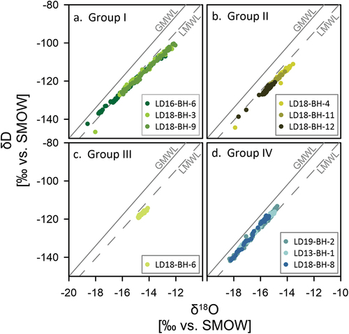
Table 8. δ¹⁸O, δD, d-excess, and EC values for both the last ice formed and for the water below the ice for different water bodies and associated separation factors ε_ice-water for oxygen and hydrogen isotopes.

Group	Water body	Core	Sample type	δ^18O (‰ vs. VSMOW)	εice-water (‰)	δD (‰ vs. VSMOW)	εice-water (‰)	d-excess (‰)	EC (μS/cm)
I	Shallow Lake	LD18-BH-3	Last ice	−16.2	2.4	−127.3	15.9	2.3	23
			Sub-ice water	−18.6		−143.2		5.6	246
		LD18-BH-9	Last ice	−16.1	2.5	−125.8	16.2	2.6	5.8
			Sub-ice water	−18.5		−142.0		6.3	223
II	Molo Lake	LD18-BH-4	Last ice	−14.8	2.5	−118.5	15.7	−0.2	4.5
			Sub-ice water	−17.2		−134.2		3.8	58
	Larisa Lake I	LD18-BH-12	Last ice	−15.8	2.6	−126.8	16.3	−0.8	8.2
			Sub-ice water	−18.4		−143.1		3.8	127.5
	Larisa Lake II	LD18-BH-11	Last ice	−15.5	2.3	−123.8	14.9	0.5	4.5
			Sub-ice water	−17.8		−138.7		3.6	69.4
III	Fish Lake	LD18-BH-6	Last ice	−14.7	2.8	−117.9	18.7	−0.4	3
			Sub-ice water	−17.5		−136.6		3.5	108.3
IV	Lena River	LD18-BH-8	Last ice	−18.2	2.8	−141.1	17.5	4.6	18.7
			Sub-ice water	−21.0		−158.6		9.1	373

Table 9. Results of ice growth simulations for each individual core compared to the actual measured ice thicknesses.

									Difference (measured vs. best-fit calculated ice thickness)
						Calculated ice thickness (best fit)			Stefan		Ashton
Group	Water body	Ice core	hs on top of the ice (m)	hs, Samoylov (m)	Measured ice thickness (m)	Stefan (m)	Ashton (m)	ρs, assumed snow density (g/cm^3)	(m)	(%)	(m)	(%)
I	Shallow Lake	LD16-BH-6	0	0.22	2.32	1.85	1.98	0.6	−0.47	20.3	−0.34	14.7
		LD18-BH-3	0	0.25	2.01	1.88	1.98	0.6	−0.13	6.5	−0.03	1.5
		LD18-BH-9	0.25	0.28	1.63	1.69	1.66	0.4	0.06	3.7	0.03	1.8
II	Molo Lake	LD18-BH-4	0	0.25	1.81	1.88	1.85	0.5	0.07	3.9	0.04	2.2
	Larisa Lake I	LD18-BH-12	0.1	0.28	2	1.9	2.01	0.6	−0.10	5.0	0.01	0.5
	Larisa Lake II	LD18-BH-11	0.1	0.28	1.83	1.9	1.87	0.5	0.07	3.8	0.04	2.2
III	Fish Lake	LD18-BH-6	0.4	0.31	1.5	1.47	1.48	0.345	−0.03	2.0	−0.02	1.3
IV	Lena River	LD13-BH-1	0.42	0.86	1.65	1.21	1.64	0.267	−0.44	26.7	−0.01	0.6
		LD18-BH-8	0.36	0.28	1.46	1.18	1.44	0.267	−0.28	19.2	−0.02	1.4
		LD19-BH-2	ca 0.2	0.18	1.76	1.08	1.75	0.267	−0.68	38.6	−0.01	0.6

Note. Samoylov snow depths are given because they served as input data for the Ashton equation. Measured snow depths on top of the ice at the time of coring are given because they were partly used to reevaluate modeling results in the discussion.

Figure 8. Isotopic snow ice signals (a) on a δ¹⁸O-δD plot and (b) in the upper 20 cm of core LD18-BH-4 (Molo Lake). Note the reflection of the isotopic snow ice signal (i.e., light δ¹⁸O values in the upper ice) in the visual ice characteristics (milky white snow ice).

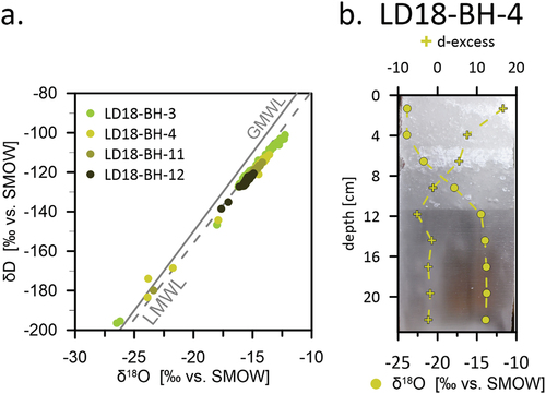
Figure 9. Results of the ice growth simulations for core LD19-BH-2 (a) and core LD16-BH-6 (b). The cores were chosen to discuss (a) the underestimation of river ice growth by Stefan and (b) the effect of using snow data of different resolutions in the Ashton equation.

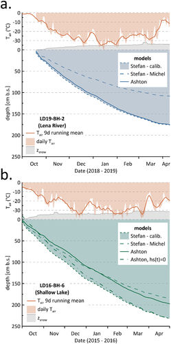
Figure 10. Differences between river water and ice chemistry. The time of freezing for ice cores was estimated using the ice growth models of Ashton. Ice chemistry is compared to water samples from the Lena Monitoring (+) and ArcticGRO (o) programs. (a) The difference in electrical conductivity (i.e., salt exclusion) over the 2018–2019 winter, (b) the same difference in EC plotted as a function of ice growth rate, (c) separation between river water and ice δ¹⁸O over the winter ice growth period (ε_ice-water = δ_ice − δ_water; see Gibson and Prowse 2002), and (d) variation of the same fractionation values (excepting the upper six ice core samples) as a function of estimated ice growth rate.

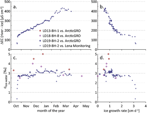
Figure 11. The stable oxygen isotope concentration in river ice (ice core LD19-BH-2) vs. interpolated values for sub-ice river water during ice growth. The linear fit is for congelation ice samples only (i.e., without the uppermost four ice core samples, gray open circles) and has the form: δ¹⁸O_ice = 0.93 δ¹⁸O_water + 1.54 (n = 75, R² = 0.96).

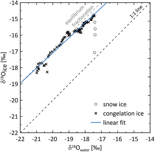
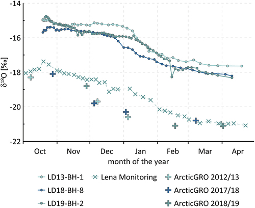
Figure 12. River ice δ¹⁸O values for all three river ice cores compared to reference data from the respective years (2012–2013, 2017–2018, and 2018–2019) provided by ArcticGRO and the Lena Monitoring Program (the latter for 2018–2019 only).

Höfle, S. T. 2015. Organic matter composition and dynamic in polygonal tundra soils. Dissertation, Universität zu Köln.

 Google Scholar

Chetverova, A., T. Skorospekhova, A. Morgenstern, N. Alekseeva, I. Spiridonov, and I. Fedorova. 2017. Hydrological and hydrochemical characteristics of lakes in the Lena River delta (Northeast-Siberia, Russia). Polarforschung 87, no. 2: 111–24. doi:10.2312/polarforschung.87.2.111.

 Google Scholar

Boike, J., C. Georgi, G. Kirilin, S. Muster, K. Abramova, I. Fedorova, A. Chetverova, M. Grigoriev, N. Bornemann, and M. Langer. 2015. Thermal processes of thermokarst lakes in the continuous permafrost zone of northern Siberia – Observations and modeling (Lena River Delta, Siberia). Biogeosciences 12, no. 20: 5941–65. doi:10.5194/bg-12-5941-2015.

 Web of Science ®Google Scholar

Morgenstern, A., G. Grosse, F. Günther, I. Fedorova, and L. Schirrmeister. 2011. Spatial analyses of thermokarst lakes and basins in Yedoma landscapes of the Lena Delta. The Cryosphere 5: 849–67. doi:10.5194/tc-5-849-2011.

 Web of Science ®Google Scholar

Morgenstern, A., C. Röhr, G. Grosse, and M. N. Grigoriev. 2011. The Lena River Delta - inventory of lakes and geomorphological terraces [dataset]. PANGAEA: Alfred Wegener Institute - Research Unit Potsdam. doi:10.1594/PANGAEA.758728.

 Google Scholar

Boike, J., J. Nitzbon, K. Anders, M. N. Grigoriev, D. Y. Bolshiyanov, M. Langer, S. Lange, et al. 2019b. Meteorologic data at station Samoylov (2002–2018, level 1, version 201908), link to archive. In: Boike, J. et al. (2019): Measurements in soil and air at Samoylov Station (2002–2018), version 201908. Alfred Wegener Institute - Research Unit Potsdam, PANGAEA, doi:10.1594/PANGAEA.905236. PANGAEA: Alfred Wegener Institute - Research Unit Potsdam. doi:10.1594/PANGAEA.905230.

 Google Scholar

Michel, B. 1971. Winter regime of rivers and lakes. Hanover, New Hampshire, U.S. Army cold regions research and engineering laboratory (CRREL). CREEL Monograph 111-B1a: 130.

 Google Scholar

Muskett, R. 2012. Remote sensing, model-derived and ground measurements of snow water equivalent and snow density in Alaska. International Journal of Geosciences 3: 1127–36. doi:10.4236/ijg.2012.35114.

 Google Scholar

Ashton, G. D. 2011. River and lake ice thickening, thinning, and snow ice formation. Cold Regions Science and Technology 68: 3–19. doi:10.1016/j.coldregions.2011.05.004.

 Web of Science ®Google Scholar

Gibson, J. J., and T. D. Prowse. 2002. Stable isotopes in river ice: Identifying primary over-winter streamflow signals and their hydrological significance. Hydrological Processes 16, no. 4: 873–90. doi:10.1002/hyp.366.

 Web of Science ®Google Scholar

Data availability statement

ArcticGro data are available via https://arcticgreatrivers.org/data/. Lena River Monitoring Program data are available at https://doi.pangaea.de/10.1594/PANGAEA.913197.