
Figures & data
Table 1. Description of the group names, treatments, and cross-fostered groups (adapted from Desaulniers et al. 2013).
Figure 1. Fold changes in Cyp genes found to be differentially expressed (FDR p ≤ 0.05; FC ≥ |1.5|) by microarray analyses in AhR, 0.5M, 0.5MAhR, and M treated groups relative to the control group at PND21. Bars are missing in absence of a statistically significant effect (data in Table S2 Loc293989 = Cyp2c6).
Figure 2. Numbers of differentially expressed genes (DEG) (FDR p ≤ 0.05; FC ≥ |1.5|) between the control and the AhR, 0.5M, 0.5MAhR, M, and the CC groups, as well as between the M and the MM group, from the microarray analyses in the male rat livers at PND21 and PND78-86. The numbers of DEG showed a dose-response effect at PND21, reflecting the amount of chemicals and TCDD-TEQ present in the mixtures (1.8, 4.1, 6.3, and 8.2 ng/kg/day TCDD-TEQ for the AhR, 0.5M, 0.5MAhR, and M groups, respectively). The groups 0.5M and 0.5MAhR at PND78-86 were not analysed by microarray.
Figure 3. Principal Component Analysis (PCA) represented by two-dimensional scatter plot (Figure 3(a,c)), and hierarchical cluster analysis (HCA) (Figure 3(b,d) based on the list of DEG (FDR p ≤ 0.05; FC ≥ |1.5|) from the comparisons of the treatment groups at PND21 (Figure 3(a,b), and at PND78-86 (Figure 3(c,d). Treatment groups were manually circled to facilitate identification and clustering in the PCA plots. In the hierarchical cluster analyses the rows represent the probes for genes with increased (red) and decreased (green) expressions (black unchanged relative to controls).
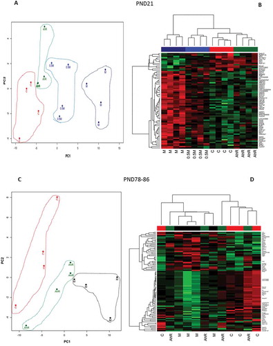
Figure 4. Venn diagram illustrating DEG (FDR p ≤ 0.05; FC ≥ |1.5|) in the comparisons of group (a) CC vs C, M vs C, and MM vs M at PND21; and (b) CC vs C, M vs C, and MM vs M at PND78-86. In Fig. 4A, the 14 genes in region “a” were: Akr1c1, Akr1c12, Arntl, Cyp2d3, Cyp2j3, Dbp, Hsd17b6, Loc689316, Lcn2, Ppapdc1a, Retsat, Rup2, Tff3, Tpt1. The two genes in region “b” were Cyp2c7 and Ubd, while the 42 genes in region “c” were: Abcb11, Actn3, Ccl21, Cmya5, Cox8b, Cpa1, Cpa2, Cpb1, Cpt1b, Cryab, Ctrb1, Des, Eno3, Fabp3, Fdps, Fgb, Fhl1, Gck, Hamp, Hrc, Igtp, Jsrp1, Klkb1, Loc688173, Lmod2, Mgc108823, Mb, Myh8, Myl4, Mylpf, Pla2g1b, Ppp1r1a, Rnase1, Slc25a30, Slc35c2, Spink3, Tnnc1, Tnnc2, Tnni2, Tnnt1, Tpm1, Upk1b. Region “d” included Sult1b1 and region “e” included 53 genes: A2m, Alas1, Aldh1a1, Aldh1a7, Aldh1b1, Apoa2, Ces1c, Ces2a, Ces2i, Ces2j, Cesl1, Cyb5a, Cyp17a1, Cyp1a1, Cyp1a2, Cyp2a1, Cyp2a3, Cyp2b2, Cyp2c37, Cyp3a23/3a1, Defa10, Entpd5, Ephx1, Gsta3, Gsta4, Gsta5, Gstm2, Loc100359554, Loc293989, Loc310902, Loc494499, Loc680955, Maged2, Mmd2, Nat8, Nfil3, Nqo1, Nr0b2, Onecut1, Pbld, Pir, Prkcdbp, Rgd1564906, Ratnp-3b, Selenbp1, Slc16a11, Slc34a2, Tsku, Ugt1a6, Ugt2a3, Ugt2b1, Ugt2b37. In Figure 4(b), the 16 genes in region “a” were: Aldh1a7, Cyp2b2, Cyp2c12, Fgl1, Hbb-b1, Inhbc, Loc305806, Loc689316, Oas1a, Oas1k, Pcolce, Rt1-n1, Rab17, Srd5a1, Tfr2, Wfdc3. The ten genes in region “b” were: Acot5, Apoa5, B3galt1, Cdh17, Dbp, Rgd1560527, Rt1Aa, Slc13a5, Sult2al1, Ubd. The two genes in region “c” were Akr1c12 and Akr1c2 while the one in region “d” was Slc35c2. Finally, the 59 genes in region “e” were: Abcg5, Acsm3, Akr1c1, Bhlha15, C6, Casp12, Cav1, Cidea, Ctnnal1, Ctnnd1, Cyp4a2, Dcn, Dusp26, Efemp1, Efna1, Eif4ebp3, Esm1, F9, Fabp4, Fam111a, Fgf21, Frzb, Gfra1, Gfra2, Gpm6a, Gpsm1, Hist1h1d, Hspa1b, Hspb1, Igfbp6, Inmt, Isg20, Kcnk2, Loc287167, Loc310926, Loc501437, Loc678704, Loc690226, Loc690435, Lox, Lrp5, Ltc4s, Mlc1, Myo7b, Nfatc4, Nrarp, Parp14, Psd, Rgd1561849, Rgd1564865, Rt1-bb, Rgs4, Sdr16c6, Serpinb7, Tap2, Thumpd1, Tpd52l1, Usp9x, Vom2r34.
Figure 5. Principal Component Analysis (PCA) represented by two-dimensional scatter plot (Figure 5(a,c), and hierarchical cluster analysis (Figure 5(b,d) using the DEG (FDR p ≤ 0.05; FC ≥ |1.5|). The DEG lists were derived from the comparisons of the treatment groups CC vs C and MM vs M at PND21 (Figure 5A and B); and CC vs C and MM vs M at PND78-86 (Figure 5(c,d). Treatment groups were manually circled to facilitate identification and clustering in the PCA plots. In the hierarchical cluster analyses the rows represent the probes for genes with increases (red) and decreases (green) in expression (black unchanged relative to controls).
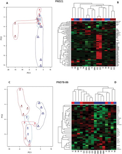
Table 2. Significant canonical pathways (CP) and upstream regulators (UR in bold) identified from DEG (FDR p ≤ 0.05 and FC ≥ |1.5|) in PND21 M rat livers. Arrows indicate if the DEG were up (↑), or down (↓) regulated.
Table 2. (Continued.)
Table 3. Top functions identified by gene networks, and canonical pathway (CP), associated with DEG (FDR p ≤ 0.05 and FC ≥ |1.5|) in the liver of M treated rat at PND21 and PND78-86. Arrow represents up (↑) or down (↓) regulation
Table 4. Top functions identified by gene networks, canonical pathway (CP), and upstream regulators (UR, bold), respectively, associated with DEG (FDR p ≤ 0.05 and FC ≥ |1.5|) in the livers of CC rats at PND21 and PND78-86. Arrows represent up (↑) or down (↓) regulation
Table 5. Top functions identified by gene networks and canonical pathway (CP), associated with DEG (FDR p ≤ 0.05 and FC ≥ |1.5|) in the livers of cross-fostered M treated rats at PND21 and PND78-86. Arrows represent up (↑) or down (↓) regulation.