Estimation and Uncertainties of Profiles and Equilibria for Fusion Modeling Codes

Figures & data

Fig. 1. (a) Profiles of the electron temperature $T_{\mathrm{e}}$, density $n_{\mathrm{e}},$ and pressure $p_{\mathrm{e}}$ profiles; (b) the corresponding gradients with respect to ${\rho }_{\mathrm{p}\mathrm{o}\mathrm{l}}$; and (c) the logarithmic gradient

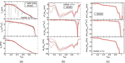
Fig. 2. Scale-length function used for nonstationary GPR

Fig. 3. (a) Profiles of the measured and estimated ion temperature $T_{\mathrm{i}}$, (b) the corresponding gradient, and (c) the logarithmic gradient

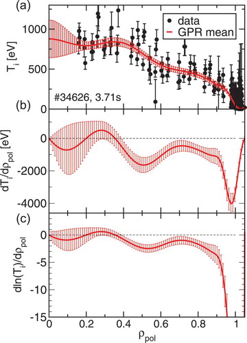
Fig. 4. (a) Candidate profiles of the ion temperature $T_{\mathrm{i}}$, (b) the corresponding gradient, and (c) the logarithmic gradient from sampling the conditional distributions

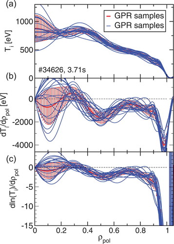
Fig. 5. (a) Profiles of the measured and estimated angular velocity $v_{\mathrm{t}\mathrm{o}\mathrm{r}},$ (b) the corresponding gradient, and (c) the logarithmic gradient

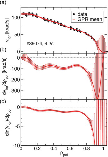
Fig. 6. (a) Candidate profiles of the angular velocity $v_{\mathrm{t}\mathrm{o}\mathrm{r}},$ (b) the corresponding gradient, and (c) the logarithmic gradient from sampling the conditional distributions

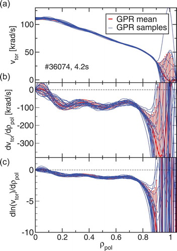
Fig. 7. Effective ion charge $Z_{\mathrm{e}\mathrm{f}\mathrm{f}}$ as a function of time including uncertainty

Fig. 8. Poloidal view of magnetic equilibria evaluated with magnetic measurements only (blue) and with additional kinetic constraints and current diffusion modeling (red)

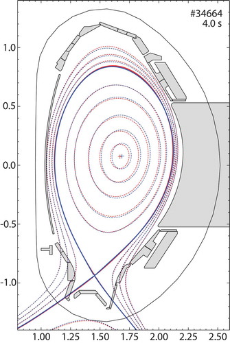
Fig. 9. Comparison of the radial position of the magnetic axis evaluated with magnetic measurements only (CLISTE mag, blue); magnetic and plasma edge thermal pressure (kinetic) constraints (CLISTE kin, green); and with magnetic, full (thermal and fast-ion) pressure constraints and current diffusion modeling (IDE, red lines with upper and lower 1σ uncertainty band)

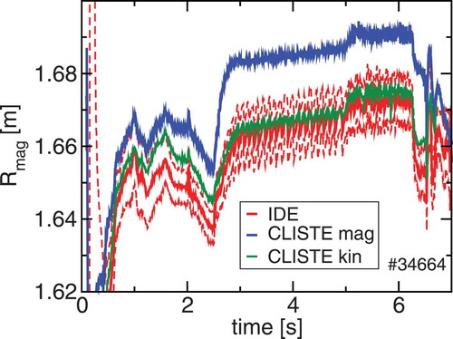
Fig. 10. Comparison of the plasma energy $W_{\mathrm{m}\mathrm{h}\mathrm{d}}$ and internal inductance $l_{\mathrm{i}}$ evaluated with magnetic measurements only (CLISTE mag, blue); magnetic and plasma edge thermal pressure (kinetic) constraints (CLISTE kin, green); and with magnetic, full (thermal and fast-ion) pressure constraints and current diffusion modeling (IDE, red)

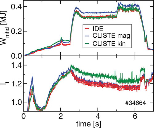
Fig. 11. Current density profile estimated applying constraints from the CDE. The uncertainties are calculated without (blue) and with (red) current constraint included

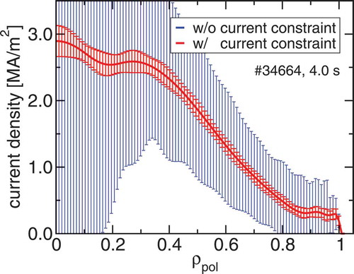
Fig. 12. The $q$-profile estimated applying constraints from the CDE. The uncertainties are calculated without (blue) and with (red) current constraint included

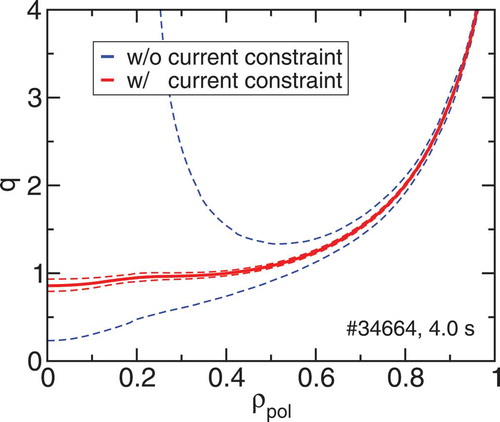
Fig. 13. Separatrix contours and poloidal coordinate system to unwrap the distance of two separatrices

Fig. 14. Toroidal location of two poloidal field coil arrays

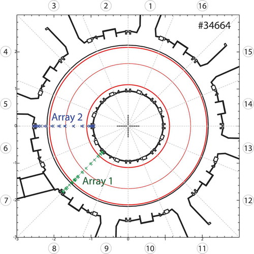
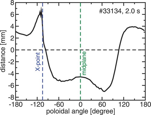
Fig. 15. Distance between the separatrices evaluated with either poloidal field coil array 1 or array 2

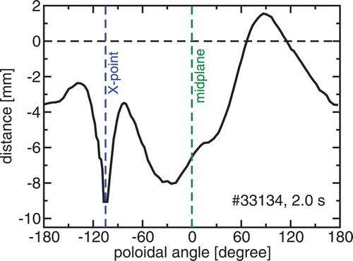
Fig. 16. Temporal evolution of the plasma volume comparing two equilibria using poloidal field array 1 or array 2

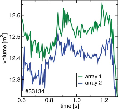
Fig. 17. Temporal evolution of the plasma current comparing two equilibria using poloidal field array 1 or array 2

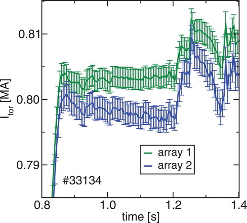
Fig. 18. Distance between the separatrices evaluated with less uncertainty in the fitting of the currents in the poloidal field coils compared to allowing for more flexibility to address uncertainties in the current measurements and induced vessel current