Numerical simulation of deployable ultra-thin composite shell structures for space applications and comparison with experiments

Figures & data

Figure 1. Deployment phase of a TRAC.

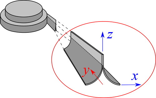
Figure 2. Deployment phase of a tape-spring.

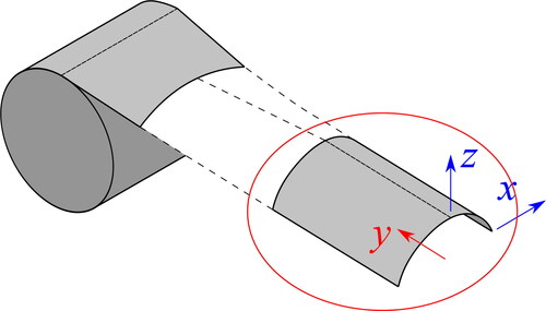
Figure 3. One-dimensional model of the TRAC.

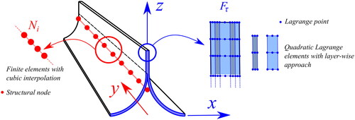
Figure 4. One-dimensional model of the tape-spring.

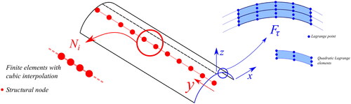
Figure 5. Geometry and stacking sequence of the composite TRAC subjected to positive and negative moments M_x. The blue color indicates the CF layers, the red color indicates the CFPW material.

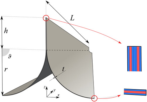
Table 1. Material properties of the composite TRAC.

	E1	E2	G12	ν12	t${}_{\text{layer}}$
	(GPa)	(GPa)	(GPa)	(-)	(μm)
CF	128	6.5	7.6	0.35	30
GFPW	23.8	23.8	3.3	0.17	25

Figure 6. Nonlinear static solution for the composite TRAC subjected to positive and negative moments M_x.

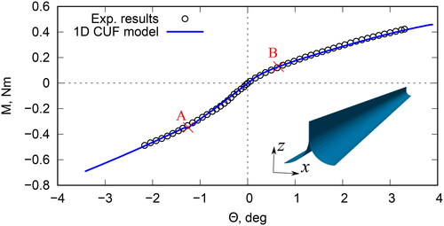
Figure 7. Nonlinear equilibrium states correspondent to the point “A” of Figure 6 for the composite TRAC subjected to a negative moment M_x. Numerical (a) vs. experimental (b) solutions (elaborated from Ref. [49]).

Figure 8. Nonlinear equilibrium states correspondent to the point “B” of Figure 6 for the composite TRAC subjected to a positive moment M_x. Numerical (a) vs. experimental (b) solutions (elaborated from Ref. [49]).

Figure 9. Nonlinear static solution for the composite TRAC subjected to positive and negative moments M_x considering the $[\pm {45}_{\text{GFWP}}/{45}_{\text{CF}}/\pm {45}_{\text{GFWP}}]$ and $[\pm {45}_{\text{GFWP}}/{90}_{\text{CF}}/\pm {45}_{\text{GFWP}}]$ stacking sequences.

Figure 10. Nonlinear equilibrium states correspondent to the buckling of the $[\pm {45}_{\text{GFWP}}/{45}_{\text{CF}}/\pm {45}_{\text{GFWP}}]$ TRAC subjected to negative (a) and positive (b) moments M_x. The equilibrium states correspond to the red circled of the Figure 9.

Figure 11. Nonlinear equilibrium states correspondent to the buckling of the $[\pm {45}_{\text{GFWP}}/{90}_{\text{CF}}/\pm {45}_{\text{GFWP}}]$ TRAC subjected to negative (a) and positive (b) moments M_x. The equilibrium states correspond to the gray circled of the Figure 9.

Figure 12. Geometry of the isotropic tape.

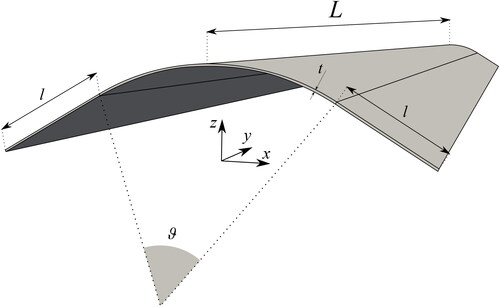
Figure 13. A 170 mm sample of commercial tape-spring. Figure elaborated from Ref. [39].

Figure 14. Nonlinear static solution for the isotropic tape subjected to positive and negative moments M_x.

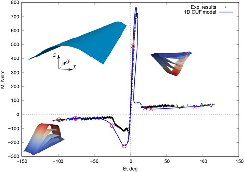
Figure 15. Nonlinear equilibrium states correspondent to crosses of Figure 14 for the isotropic tape subjected to a positive moment M_x. Numerical (a) vs. experimental (b) solutions, elaborated from Ref. [39].

Figure 16. Nonlinear equilibrium states correspondent to circles of Figure 14 for the isotropic tape subjected to a positive moment M_x. Numerical (a) vs. experimental (b) solutions, elaborated from Ref. [39].

Figure 17. Nonlinear static solution for the isotropic tape using a defect load.

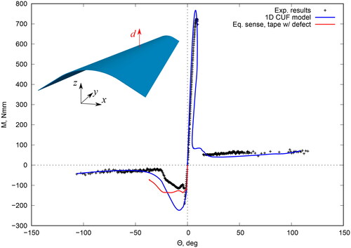
Figure 18. Nonlinear equilibrium states correspondent to crosses of Figure 14 for the isotropic tape subjected to a positive moment M_x, using a defect load for the numerical simulations. Experimental figures elaborated from Ref. [39].

C. Leclerc and S. Pellegrino, Nonlinear elastic buckling of ultra-thin coilable booms, Int. J. Solids Struct., vol. 203, pp. 46–56, 2020. DOI: 10.1016/j.ijsolstr.2020.06.042.

 Web of Science ®Google Scholar

A. Pagani, E. Carrera, A. G. de Miguel, A. Hasanyan, S. Pellegrino, H. R. Narravula, E. Zappino, Efficient analysis of geometrically nonlinear deployable thin shell structures using Carrera unified formulation, 70th International Astronautical Congress (IAC), Washington D.C., USA, 2019.

 Google Scholar