Stiffness and stress fluctuations in dental cement paste: a continuum micromechanics approach

Figures & data

Figure 1. Histogram of indentation modulus approximated by the superposition of three lognormal distributions; after [3].

Table 1. Results obtained from grid nanoindentation testing [3]: values of medians, modes, and volume fractions associated with the three lognormal distributions representing the histogram of indentation moduli in Fig. 1.

Lognormal distribution	Median [GPa]	Mode [GPa]	Volume fraction [–]
LDCR hydrates	45.1	24.5	0.1228
HDCR hydrates	62.6	60.2	0.7420
clinker and zirconia	92.2	89.0	0.1352
		sum:	1.0000

Table 2. Input quantities of the solid material constituents: bulk moduli, k_i, shear moduli g_i, as well as lognormal parameters μ_i and σ_i which are consistent with median and mode values listed in Table 1; input values taken from [3, 17, 18].

Phase	Index	Stiffness properties		Volume fraction
zirconia	i = 1	$k_1=170.8$ GPa	$g_1=78.8$ GPa	$f_1=0.0182$
clinker	i = 2	$k_2=116.7$ GPa	$g_2=53.8$ GPa	$f_2=0.1170$
HDCR hydrates	i = 3	${\mu }_3=4.14$	${\sigma }_3=0.20$	$f_3=0.7420$
LDCR hydrates	i = 4	${\mu }_4=3.81$	${\sigma }_4=0.78$	$f_4=0.1228$

Figure 2. Micromechanical representation of Biodentine (“material organogram”): the two-dimensional sketch shows qualitative properties of a three-dimensional representative volume element of the lognormal microelasticity model which accounts for stiffness distributions of two populations of hydrates.

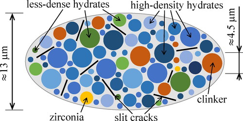
Figure 3. Eshelby-type matrix inclusion problems: (a) spherical inclusion, and (b) oblate spheroid, both embedded in an infinite matrix with isotropic stiffness ${\mathrm{C}}_{\mathit{bio}}$, subjected remotely to auxiliary uniform strains ${\mathbf{E}}_{\infty }.$

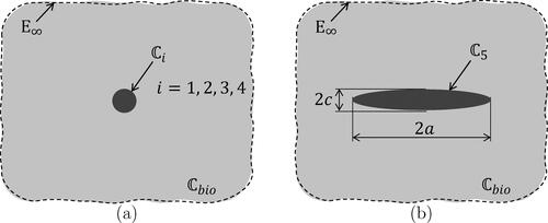
Figure 4. Thin oblate spheroid oriented in ψ,ϑ-direction.

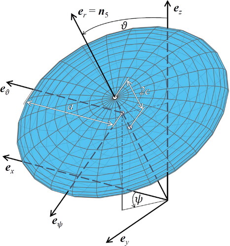
Figure 5. (a) Bulk and (b) shear modulus of the hydrates as a function of the indentation modulus, for three different values of Poisson’s ratio of the hydrates.

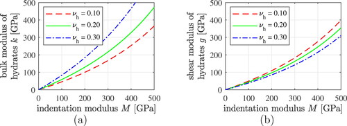
Table 3. Flowchart for the computation of k_bio and g_bio according to Eqs. (41)(41) $$\begin{array}{c}{k}_{\mathit{bio}}=\{\sum _{i=1}^2\frac{f_i{k}_i}{1+\frac{S_{\mathit{vol}}(k_i-k_{\mathit{bio}})}{k_{\mathit{bio}}}}+\sum _{i=3}^4{f}_i\underset{0}{\overset{\infty }{\int }}\frac{{\phi }_i(M)k_i(M)}{1+\frac{S_{\mathit{vol}}(k_i(M)-k_{\mathit{bio}})}{k_{\mathit{bio}}}} \mathrm{d}M\}\\ \times {\{\sum _{i=1}^2\frac{f_i}{1+\frac{S_{\mathit{vol}}(k_i-k_{\mathit{bio}})}{k_{\mathit{bio}}}}+\sum _{i=3}^4{f}_i\mathrm{ }\underset{0}{\overset{\infty }{\int }}\frac{{\phi }_i(M)}{1+\frac{S_{\mathit{vol}}(k_i(M)-k_{\mathit{bio}})}{k_{\mathit{bio}}}} \mathrm{d}M\}}^{-1},\end{array}$$(41) and (42)(42) $$\begin{array}{c}{g}_{\mathit{bio}}=\{\sum _{i=1}^2\frac{f_i{g}_i}{1+\frac{S_{\mathit{dev}}(g_i-g_{\mathit{bio}})}{g_{\mathit{bio}}}}+\sum _{i=3}^4{f}_i\underset{0}{\overset{\infty }{\int }}\frac{{\phi }_i(M)g_i(M)}{1+\frac{S_{\mathit{dev}}(g_i(M)-g_{\mathit{bio}})}{g_{\mathit{bio}}}} \mathrm{d}M\}\\ \times \{\sum _{i=1}^2\frac{f_i}{1+\frac{S_{\mathit{dev}}(g_i-g_{\mathit{bio}})}{g_{\mathit{bio}}}}+\sum _{i=3}^4{f}_i\underset{0}{\overset{\infty }{\int }}\frac{{\phi }_i(M)}{1+\frac{S_{\mathit{dev}}(g_i(M)-g_{\mathit{bio}})}{g_{\mathit{bio}}}} \mathrm{d}M\\ \hspace{1em}+\frac{4\pi \omega }{3}{T}_{\mathit{dev}}{\}}^{-1}.\end{array}$$(42) , respectively.

1.	Define numerical values of the crack density parameter ω and of Poisson’s ratio of the hydrates, νh.
2.	Define initial values of kbio and gbio as arbitrary positive numbers; for example, $k_{\mathit{bio}}=4.2\text{GPa}$ and $g_{\mathit{bio}}=2.5\text{GPa}.$
3.	Set the tolerance value tol equal to ${10}^{-10}.$
4.	Save kbio as $k_{\mathit{bio}}^{\mathit{old}}$ and gbio as $g_{\mathit{bio}}^{\mathit{old}}.$
5.	Compute Tdev, Svol, Sdev according to Eqs. (35)(35) $$T_{\mathit{dev}}=\frac{8(3k_{\mathit{bio}}+4g_{\mathit{bio}})}{15\pi (3k_{\mathit{bio}}+2g_{\mathit{bio}})}.$$(35) , (39)(39) $$S_{\mathit{vol}}=\frac{3k_{\mathit{bio}}}{3k_{\mathit{bio}}+4g_{\mathit{bio}}},$$(39) , (40)(40) $$S_{\mathit{dev}}=\frac{6(k_{\mathit{bio}}+2g_{\mathit{bio}})}{5(3k_{\mathit{bio}}+4g_{\mathit{bio}})}.$$(40) .
6.	Evaluate the integrals in Eqs. (41)(41) $$\begin{array}{c}{k}_{\mathit{bio}}=\{\sum _{i=1}^2\frac{f_i{k}_i}{1+\frac{S_{\mathit{vol}}(k_i-k_{\mathit{bio}})}{k_{\mathit{bio}}}}+\sum _{i=3}^4{f}_i\underset{0}{\overset{\infty }{\int }}\frac{{\phi }_i(M)k_i(M)}{1+\frac{S_{\mathit{vol}}(k_i(M)-k_{\mathit{bio}})}{k_{\mathit{bio}}}} \mathrm{d}M\}\\ \times {\{\sum _{i=1}^2\frac{f_i}{1+\frac{S_{\mathit{vol}}(k_i-k_{\mathit{bio}})}{k_{\mathit{bio}}}}+\sum _{i=3}^4{f}_i\mathrm{ }\underset{0}{\overset{\infty }{\int }}\frac{{\phi }_i(M)}{1+\frac{S_{\mathit{vol}}(k_i(M)-k_{\mathit{bio}})}{k_{\mathit{bio}}}} \mathrm{d}M\}}^{-1},\end{array}$$(41) and (42)(42) $$\begin{array}{c}{g}_{\mathit{bio}}=\{\sum _{i=1}^2\frac{f_i{g}_i}{1+\frac{S_{\mathit{dev}}(g_i-g_{\mathit{bio}})}{g_{\mathit{bio}}}}+\sum _{i=3}^4{f}_i\underset{0}{\overset{\infty }{\int }}\frac{{\phi }_i(M)g_i(M)}{1+\frac{S_{\mathit{dev}}(g_i(M)-g_{\mathit{bio}})}{g_{\mathit{bio}}}} \mathrm{d}M\}\\ \times \{\sum _{i=1}^2\frac{f_i}{1+\frac{S_{\mathit{dev}}(g_i-g_{\mathit{bio}})}{g_{\mathit{bio}}}}+\sum _{i=3}^4{f}_i\underset{0}{\overset{\infty }{\int }}\frac{{\phi }_i(M)}{1+\frac{S_{\mathit{dev}}(g_i(M)-g_{\mathit{bio}})}{g_{\mathit{bio}}}} \mathrm{d}M\\ \hspace{1em}+\frac{4\pi \omega }{3}{T}_{\mathit{dev}}{\}}^{-1}.\end{array}$$(42) based on ${\phi }_3(M)$ and ${\phi }_4(M)$ according to Eq. (19)(19) $${\phi }_i(M)=\frac{1}{M{\sigma }_i\sqrt{2\pi }}\hspace{0.17em}\text{exp}\hspace{0.17em}\mathrm{}(\mathrm{}-\frac{1}{2}{\left[\frac{\hspace{0.17em}\text{ln}\hspace{0.17em}(M)-{\mu }_i}{{\sigma }_i}\right]}^2),\hspace{1em}i=3,4.$$(19) with values of μ3, σ3, μ4, σ4 from Table 2, as well as $k_3(M),g_3(M),k_4(M),g_4(M)$ according to Eqs. (57)(57) $$k_i(M)=\frac{E(M)}{3(1-2{\nu }_h)},\hspace{1em}i=3,4,$$(57) and (58)(58) $$g_i(M)=\frac{E(M)}{2(1+{\nu }_h)},\hspace{1em}i=3,4,$$(58) , with E(M) according to Eq. (56)(56) $$E(M)=\frac{1-{\nu }_h^2}{\frac{1}{M}-\frac{1-{0.07}^2}{1141\text{GPa}}}.$$(56) .
7.	Evaluate the sums in Eqs. (41)(41) $$\begin{array}{c}{k}_{\mathit{bio}}=\{\sum _{i=1}^2\frac{f_i{k}_i}{1+\frac{S_{\mathit{vol}}(k_i-k_{\mathit{bio}})}{k_{\mathit{bio}}}}+\sum _{i=3}^4{f}_i\underset{0}{\overset{\infty }{\int }}\frac{{\phi }_i(M)k_i(M)}{1+\frac{S_{\mathit{vol}}(k_i(M)-k_{\mathit{bio}})}{k_{\mathit{bio}}}} \mathrm{d}M\}\\ \times {\{\sum _{i=1}^2\frac{f_i}{1+\frac{S_{\mathit{vol}}(k_i-k_{\mathit{bio}})}{k_{\mathit{bio}}}}+\sum _{i=3}^4{f}_i\mathrm{ }\underset{0}{\overset{\infty }{\int }}\frac{{\phi }_i(M)}{1+\frac{S_{\mathit{vol}}(k_i(M)-k_{\mathit{bio}})}{k_{\mathit{bio}}}} \mathrm{d}M\}}^{-1},\end{array}$$(41) and (42)(42) $$\begin{array}{c}{g}_{\mathit{bio}}=\{\sum _{i=1}^2\frac{f_i{g}_i}{1+\frac{S_{\mathit{dev}}(g_i-g_{\mathit{bio}})}{g_{\mathit{bio}}}}+\sum _{i=3}^4{f}_i\underset{0}{\overset{\infty }{\int }}\frac{{\phi }_i(M)g_i(M)}{1+\frac{S_{\mathit{dev}}(g_i(M)-g_{\mathit{bio}})}{g_{\mathit{bio}}}} \mathrm{d}M\}\\ \times \{\sum _{i=1}^2\frac{f_i}{1+\frac{S_{\mathit{dev}}(g_i-g_{\mathit{bio}})}{g_{\mathit{bio}}}}+\sum _{i=3}^4{f}_i\underset{0}{\overset{\infty }{\int }}\frac{{\phi }_i(M)}{1+\frac{S_{\mathit{dev}}(g_i(M)-g_{\mathit{bio}})}{g_{\mathit{bio}}}} \mathrm{d}M\\ \hspace{1em}+\frac{4\pi \omega }{3}{T}_{\mathit{dev}}{\}}^{-1}.\end{array}$$(42) based on f1, f2, f3, f4, k1, g1, k2, g2 from Table 2.
8.	Quantify kbio and gbio according to Eqs. (41)(41) $$\begin{array}{c}{k}_{\mathit{bio}}=\{\sum _{i=1}^2\frac{f_i{k}_i}{1+\frac{S_{\mathit{vol}}(k_i-k_{\mathit{bio}})}{k_{\mathit{bio}}}}+\sum _{i=3}^4{f}_i\underset{0}{\overset{\infty }{\int }}\frac{{\phi }_i(M)k_i(M)}{1+\frac{S_{\mathit{vol}}(k_i(M)-k_{\mathit{bio}})}{k_{\mathit{bio}}}} \mathrm{d}M\}\\ \times {\{\sum _{i=1}^2\frac{f_i}{1+\frac{S_{\mathit{vol}}(k_i-k_{\mathit{bio}})}{k_{\mathit{bio}}}}+\sum _{i=3}^4{f}_i\mathrm{ }\underset{0}{\overset{\infty }{\int }}\frac{{\phi }_i(M)}{1+\frac{S_{\mathit{vol}}(k_i(M)-k_{\mathit{bio}})}{k_{\mathit{bio}}}} \mathrm{d}M\}}^{-1},\end{array}$$(41) and (42)(42) $$\begin{array}{c}{g}_{\mathit{bio}}=\{\sum _{i=1}^2\frac{f_i{g}_i}{1+\frac{S_{\mathit{dev}}(g_i-g_{\mathit{bio}})}{g_{\mathit{bio}}}}+\sum _{i=3}^4{f}_i\underset{0}{\overset{\infty }{\int }}\frac{{\phi }_i(M)g_i(M)}{1+\frac{S_{\mathit{dev}}(g_i(M)-g_{\mathit{bio}})}{g_{\mathit{bio}}}} \mathrm{d}M\}\\ \times \{\sum _{i=1}^2\frac{f_i}{1+\frac{S_{\mathit{dev}}(g_i-g_{\mathit{bio}})}{g_{\mathit{bio}}}}+\sum _{i=3}^4{f}_i\underset{0}{\overset{\infty }{\int }}\frac{{\phi }_i(M)}{1+\frac{S_{\mathit{dev}}(g_i(M)-g_{\mathit{bio}})}{g_{\mathit{bio}}}} \mathrm{d}M\\ \hspace{1em}+\frac{4\pi \omega }{3}{T}_{\mathit{dev}}{\}}^{-1}.\end{array}$$(42) .
9.	Determine the convergence ratio according to $c=\frac{\Vert k_{\mathit{bio}}-k_{\mathit{bio}}^{\mathit{old}}\Vert }{k_{\mathit{bio}}^{\mathit{old}}}+\frac{\Vert g_{\mathit{bio}}-g_{\mathit{bio}}^{\mathit{old}}\Vert }{g_{\mathit{bio}}^{\mathit{old}}}.$
10.	If c < tol then stop the iteration; else go to 4. (= start the next iteration step).

Figure 6. Square root of the sum of squared errors (59), quantifying the difference between computed homogenized stiffness moduli, see Eqs. (41)(41) $$\begin{array}{c}{k}_{\mathit{bio}}=\{\sum _{i=1}^2\frac{f_i{k}_i}{1+\frac{S_{\mathit{vol}}(k_i-k_{\mathit{bio}})}{k_{\mathit{bio}}}}+\sum _{i=3}^4{f}_i\underset{0}{\overset{\infty }{\int }}\frac{{\phi }_i(M)k_i(M)}{1+\frac{S_{\mathit{vol}}(k_i(M)-k_{\mathit{bio}})}{k_{\mathit{bio}}}} \mathrm{d}M\}\\ \times {\{\sum _{i=1}^2\frac{f_i}{1+\frac{S_{\mathit{vol}}(k_i-k_{\mathit{bio}})}{k_{\mathit{bio}}}}+\sum _{i=3}^4{f}_i\mathrm{ }\underset{0}{\overset{\infty }{\int }}\frac{{\phi }_i(M)}{1+\frac{S_{\mathit{vol}}(k_i(M)-k_{\mathit{bio}})}{k_{\mathit{bio}}}} \mathrm{d}M\}}^{-1},\end{array}$$(41) and (42)(42) $$\begin{array}{c}{g}_{\mathit{bio}}=\{\sum _{i=1}^2\frac{f_i{g}_i}{1+\frac{S_{\mathit{dev}}(g_i-g_{\mathit{bio}})}{g_{\mathit{bio}}}}+\sum _{i=3}^4{f}_i\underset{0}{\overset{\infty }{\int }}\frac{{\phi }_i(M)g_i(M)}{1+\frac{S_{\mathit{dev}}(g_i(M)-g_{\mathit{bio}})}{g_{\mathit{bio}}}} \mathrm{d}M\}\\ \times \{\sum _{i=1}^2\frac{f_i}{1+\frac{S_{\mathit{dev}}(g_i-g_{\mathit{bio}})}{g_{\mathit{bio}}}}+\sum _{i=3}^4{f}_i\underset{0}{\overset{\infty }{\int }}\frac{{\phi }_i(M)}{1+\frac{S_{\mathit{dev}}(g_i(M)-g_{\mathit{bio}})}{g_{\mathit{bio}}}} \mathrm{d}M\\ \hspace{1em}+\frac{4\pi \omega }{3}{T}_{\mathit{dev}}{\}}^{-1}.\end{array}$$(42) as well as Table 3, and their experimental counterparts, see Eqs. (1)(1) $$k_{\mathit{bio}}^{\hspace{0.17em}\mathit{\text{exp}}\hspace{0.17em}}=38.4\text{GPa},$$(1) and (2)(2) $$g_{\mathit{bio}}^{\hspace{0.17em}\mathit{\text{exp}}\hspace{0.17em}}=14.1\text{GPa},$$(2) .

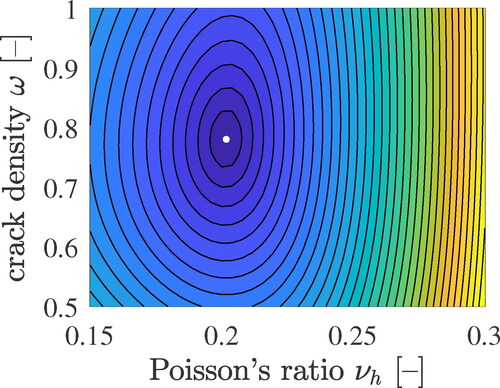
Figure 7. Homogenized stiffness moduli k_bio and g_bio according to Eqs. (41)(41) $$\begin{array}{c}{k}_{\mathit{bio}}=\{\sum _{i=1}^2\frac{f_i{k}_i}{1+\frac{S_{\mathit{vol}}(k_i-k_{\mathit{bio}})}{k_{\mathit{bio}}}}+\sum _{i=3}^4{f}_i\underset{0}{\overset{\infty }{\int }}\frac{{\phi }_i(M)k_i(M)}{1+\frac{S_{\mathit{vol}}(k_i(M)-k_{\mathit{bio}})}{k_{\mathit{bio}}}} \mathrm{d}M\}\\ \times {\{\sum _{i=1}^2\frac{f_i}{1+\frac{S_{\mathit{vol}}(k_i-k_{\mathit{bio}})}{k_{\mathit{bio}}}}+\sum _{i=3}^4{f}_i\mathrm{ }\underset{0}{\overset{\infty }{\int }}\frac{{\phi }_i(M)}{1+\frac{S_{\mathit{vol}}(k_i(M)-k_{\mathit{bio}})}{k_{\mathit{bio}}}} \mathrm{d}M\}}^{-1},\end{array}$$(41) and (42)(42) $$\begin{array}{c}{g}_{\mathit{bio}}=\{\sum _{i=1}^2\frac{f_i{g}_i}{1+\frac{S_{\mathit{dev}}(g_i-g_{\mathit{bio}})}{g_{\mathit{bio}}}}+\sum _{i=3}^4{f}_i\underset{0}{\overset{\infty }{\int }}\frac{{\phi }_i(M)g_i(M)}{1+\frac{S_{\mathit{dev}}(g_i(M)-g_{\mathit{bio}})}{g_{\mathit{bio}}}} \mathrm{d}M\}\\ \times \{\sum _{i=1}^2\frac{f_i}{1+\frac{S_{\mathit{dev}}(g_i-g_{\mathit{bio}})}{g_{\mathit{bio}}}}+\sum _{i=3}^4{f}_i\underset{0}{\overset{\infty }{\int }}\frac{{\phi }_i(M)}{1+\frac{S_{\mathit{dev}}(g_i(M)-g_{\mathit{bio}})}{g_{\mathit{bio}}}} \mathrm{d}M\\ \hspace{1em}+\frac{4\pi \omega }{3}{T}_{\mathit{dev}}{\}}^{-1}.\end{array}$$(42) , as functions of the crack density of Biodentine and Poisson’s ratio of the hydrates, see the solid blue lines, and ultrasonics-derived counterparts according to Eqs. (1)(1) $$k_{\mathit{bio}}^{\hspace{0.17em}\mathit{\text{exp}}\hspace{0.17em}}=38.4\text{GPa},$$(1) and (2)(2) $$g_{\mathit{bio}}^{\hspace{0.17em}\mathit{\text{exp}}\hspace{0.17em}}=14.1\text{GPa},$$(2) , see the red dashed lines; the circles mark the optimal solutions, see also Eqs. (60)(60) $$\omega =0.7802,$$(60) and (61)(61) $${\nu }_h=0.2017,$$(61) .

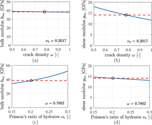
Figure 8. Results of the lognormal microelasticity model (black graphs): statistical distributions of volumetric and deviatoric components of the strain concentration tensors of LDCR hydrates and of HDCR hydrates: (a) and (c) show probability density distributions, (b) and (d) cumulative distribution functions. The best fits of generalized beta-distributions to the statistical distributions are the red dashed graphs, see Eqs. (70)(70) $${\phi }_i^B(y)=\frac{{\left(\frac{y-a}{c-a}\right)}^{\alpha -1}{\left(\frac{c-y}{c-a}\right)}^{\beta -1}}{(c-a)\times B(\alpha ,\beta )},$$(70) and (71)(71) $$B(\alpha ,\beta )=\frac{\Gamma (\alpha )\Gamma (\beta )}{\Gamma (\alpha +\beta )},$$(71) as well as the Beta distributions parameters listed in Table 6.

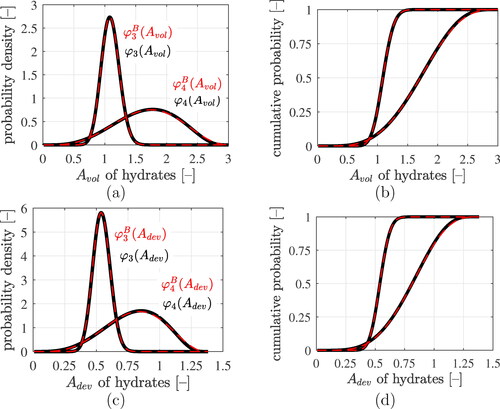
Table 4. Results of the lognormal microelasticity model: (population-averaged) strain concentration tensors components of the four types of solid constituents of Biodentine.

Constituent of Biodentine	(Average) strain concentration tensor components		Source
zirconia	$A_{\mathit{vol},1}=0.3017$	$A_{\mathit{dev},1}=0.2352$	Eqs. (44)(44) $$\begin{array}{c}{A}_{\mathit{vol},i}=\frac{1}{1+\frac{S_{\mathit{vol}}(k_i-k_{\mathit{bio}})}{k_{\mathit{bio}}}}\{\sum _{i=1}^2\frac{f_i}{1+\frac{S_{\mathit{vol}}(k_i-k_{\mathit{bio}})}{k_{\mathit{bio}}}}\\ +\sum _{i=3}^4{f}_i\mathrm{ }\underset{0}{\overset{\infty }{\int }}\frac{{\phi }_i(M)}{1+\frac{S_{\mathit{vol}}(k_i(M)-k_{\mathit{bio}})}{k_{\mathit{bio}}}} \mathrm{d}M{\}}^{-1},\end{array}$$(44) and (45)(45) $$\begin{array}{c}{A}_{\mathit{dev},i}=\frac{1}{1+\frac{S_{\mathit{dev}}(g_i-g_{\mathit{bio}})}{g_{\mathit{bio}}}}\{\sum _{i=1}^2\frac{f_i}{1+\frac{S_{\mathit{dev}}(g_i-g_{\mathit{bio}})}{g_{\mathit{bio}}}}\\ +\sum _{i=3}^4{f}_i\mathrm{ }\underset{0}{\overset{\infty }{\int }}\frac{{\phi }_i(M)}{1+\frac{S_{\mathit{dev}}(g_i(M)-g_{\mathit{bio}})}{g_{\mathit{bio}}}} \mathrm{d}M+\frac{4\pi \omega }{3}{T}_{\mathit{dev}}{\}}^{-1}.\end{array}$$(45)
clinker	$A_{\mathit{vol},2}=0.4223$	$A_{\mathit{dev},2}=0.3192$	Eqs. (44)(44) $$\begin{array}{c}{A}_{\mathit{vol},i}=\frac{1}{1+\frac{S_{\mathit{vol}}(k_i-k_{\mathit{bio}})}{k_{\mathit{bio}}}}\{\sum _{i=1}^2\frac{f_i}{1+\frac{S_{\mathit{vol}}(k_i-k_{\mathit{bio}})}{k_{\mathit{bio}}}}\\ +\sum _{i=3}^4{f}_i\mathrm{ }\underset{0}{\overset{\infty }{\int }}\frac{{\phi }_i(M)}{1+\frac{S_{\mathit{vol}}(k_i(M)-k_{\mathit{bio}})}{k_{\mathit{bio}}}} \mathrm{d}M{\}}^{-1},\end{array}$$(44) and (45)(45) $$\begin{array}{c}{A}_{\mathit{dev},i}=\frac{1}{1+\frac{S_{\mathit{dev}}(g_i-g_{\mathit{bio}})}{g_{\mathit{bio}}}}\{\sum _{i=1}^2\frac{f_i}{1+\frac{S_{\mathit{dev}}(g_i-g_{\mathit{bio}})}{g_{\mathit{bio}}}}\\ +\sum _{i=3}^4{f}_i\mathrm{ }\underset{0}{\overset{\infty }{\int }}\frac{{\phi }_i(M)}{1+\frac{S_{\mathit{dev}}(g_i(M)-g_{\mathit{bio}})}{g_{\mathit{bio}}}} \mathrm{d}M+\frac{4\pi \omega }{3}{T}_{\mathit{dev}}{\}}^{-1}.\end{array}$$(45)
HDCR hydrates	${\overline{A_{\mathit{vol}}}}_{,3}=1.0551$	${\overline{A_{\mathit{dev}}}}_{,3}=0.5248$	Eqs. (64)(64) $$\begin{array}{c}\overline{A_{\mathit{vol},j}}=\underset{0}{\overset{\infty }{\int }}\frac{{\phi }_j(M)}{1+\frac{S_{\mathit{vol}}(k_j(M)-k_{\mathit{bio}})}{k_{\mathit{bio}}}} \mathrm{d}M\\ \times {\{\sum _{i=1}^2\frac{f_i}{1+\frac{S_{\mathit{vol}}(k_i-k_{\mathit{bio}})}{k_{\mathit{bio}}}}+\sum _{i=3}^4{f}_i\mathrm{ }\underset{0}{\overset{\infty }{\int }}\frac{{\phi }_i(M)}{1+\frac{S_{\mathit{vol}}(k_i(M)-k_{\mathit{bio}})}{k_{\mathit{bio}}}} \mathrm{d}M\}}^{-1},\end{array}$$(64) and (65)(65) $$\begin{array}{c}\overline{A_{\mathit{dev},j}}=\underset{0}{\overset{\infty }{\int }}\frac{{\phi }_j(M)}{1+\frac{S_{\mathit{dev}}(g_j(M)-g_{\mathit{bio}})}{g_{\mathit{bio}}}} \mathrm{d}M\\ \times \{\sum _{i=1}^2\frac{f_i}{1+\frac{S_{\mathit{dev}}(g_i-g_{\mathit{bio}})}{g_{\mathit{bio}}}}+\sum _{i=3}^4{f}_i\mathrm{ }\underset{0}{\overset{\infty }{\int }}\frac{{\phi }_i(M)}{1+\frac{S_{\mathit{dev}}(g_i(M)-g_{\mathit{bio}})}{g_{\mathit{bio}}}} \mathrm{d}M+\frac{4\pi \omega }{3}{T}_{\mathit{dev}}{\}}^{-1}.\end{array}$$(65)
LDCR hydrates	${\overline{A_{\mathit{vol}}}}_{,4}=1.3207$	${\overline{A_{\mathit{dev}}}}_{,4}=0.6428$	Eqs. (64)(64) $$\begin{array}{c}\overline{A_{\mathit{vol},j}}=\underset{0}{\overset{\infty }{\int }}\frac{{\phi }_j(M)}{1+\frac{S_{\mathit{vol}}(k_j(M)-k_{\mathit{bio}})}{k_{\mathit{bio}}}} \mathrm{d}M\\ \times {\{\sum _{i=1}^2\frac{f_i}{1+\frac{S_{\mathit{vol}}(k_i-k_{\mathit{bio}})}{k_{\mathit{bio}}}}+\sum _{i=3}^4{f}_i\mathrm{ }\underset{0}{\overset{\infty }{\int }}\frac{{\phi }_i(M)}{1+\frac{S_{\mathit{vol}}(k_i(M)-k_{\mathit{bio}})}{k_{\mathit{bio}}}} \mathrm{d}M\}}^{-1},\end{array}$$(64) and (65)(65) $$\begin{array}{c}\overline{A_{\mathit{dev},j}}=\underset{0}{\overset{\infty }{\int }}\frac{{\phi }_j(M)}{1+\frac{S_{\mathit{dev}}(g_j(M)-g_{\mathit{bio}})}{g_{\mathit{bio}}}} \mathrm{d}M\\ \times \{\sum _{i=1}^2\frac{f_i}{1+\frac{S_{\mathit{dev}}(g_i-g_{\mathit{bio}})}{g_{\mathit{bio}}}}+\sum _{i=3}^4{f}_i\mathrm{ }\underset{0}{\overset{\infty }{\int }}\frac{{\phi }_i(M)}{1+\frac{S_{\mathit{dev}}(g_i(M)-g_{\mathit{bio}})}{g_{\mathit{bio}}}} \mathrm{d}M+\frac{4\pi \omega }{3}{T}_{\mathit{dev}}{\}}^{-1}.\end{array}$$(65)

Figure 9. Results of the lognormal microelasticity model (black graphs): statistical distributions of volumetric and deviatoric components of the stress concentration tensors of LDCR hydrates and of HDCR hydrates: (a) and (c) show probability density distributions, (b) and (d) cumulative distribution functions. The best fits of generalized beta-distributions to the statistical distributions are the red dashed graphs, see Eqs. (70)(70) $${\phi }_i^B(y)=\frac{{\left(\frac{y-a}{c-a}\right)}^{\alpha -1}{\left(\frac{c-y}{c-a}\right)}^{\beta -1}}{(c-a)\times B(\alpha ,\beta )},$$(70) and (71)(71) $$B(\alpha ,\beta )=\frac{\Gamma (\alpha )\Gamma (\beta )}{\Gamma (\alpha +\beta )},$$(71) as well as the Beta distributions parameters listed in Table 7.

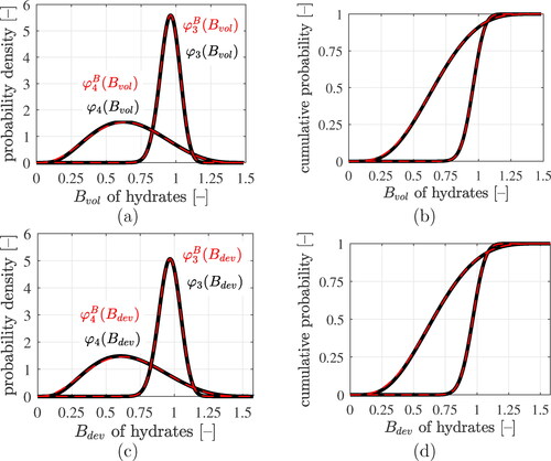
Table 5. Results of the lognormal microelasticity model: (population-averaged) stress concentration tensors components of the four types of solid constituents of Biodentine.

Constituent of Biodentine	(Average) stress concentration tensor components		Source
zirconia	$B_{\mathit{vol},1}=1.3419$	$B_{\mathit{dev},1}=1.3152$	Eqs. (49)(49) $$B_{\mathit{vol},i}=\frac{k_i}{k_{\mathit{bio}}}{A}_{\mathit{vol},i},$$(49) and (50)(50) $$B_{\mathit{dev},i}=\frac{g_i}{g_{\mathit{bio}}}{A}_{\mathit{dev},i},$$(50)
clinker	$B_{\mathit{vol},2}=1.2828$	$B_{\mathit{dev},2}=1.2188$	Eqs. (49)(49) $$B_{\mathit{vol},i}=\frac{k_i}{k_{\mathit{bio}}}{A}_{\mathit{vol},i},$$(49) and (50)(50) $$B_{\mathit{dev},i}=\frac{g_i}{g_{\mathit{bio}}}{A}_{\mathit{dev},i},$$(50)
HDCR hydrates	${\overline{B_{\mathit{vol}}}}_{,3}=0.9730$	${\overline{B_{\mathit{dev}}}}_{,3}=0.9830$	Eqs. (68)(68) $$\begin{array}{c}\overline{B_{\mathit{vol},j}}=\frac{1}{k_{\mathit{bio}}}\underset{0}{\overset{\infty }{\int }}\frac{{\phi }_j(M)k_j(M)}{1+\frac{S_{\mathit{vol}}(k_j(M)-k_{\mathit{bio}})}{k_{\mathit{bio}}}} \mathrm{d}M\\ \times {\{\sum _{i=1}^2\frac{f_i}{1+\frac{S_{\mathit{vol}}(k_i-k_{\mathit{bio}})}{k_{\mathit{bio}}}}+\sum _{i=3}^4{f}_i\mathrm{ }\underset{0}{\overset{\infty }{\int }}\frac{{\phi }_i(M)}{1+\frac{S_{\mathit{vol}}(k_i(M)-k_{\mathit{bio}})}{k_{\mathit{bio}}}} \mathrm{d}M\}}^{-1},\end{array}$$(68) and (69)(69) $$\begin{array}{c}\overline{B_{\mathit{dev},j}}=\frac{1}{g_{\mathit{bio}}}\underset{0}{\overset{\infty }{\int }}\frac{{\phi }_j(M)g_j(M)}{1+\frac{S_{\mathit{dev}}(g_j(M)-g_{\mathit{bio}})}{g_{\mathit{bio}}}} \mathrm{d}M\\ \times \{\sum _{i=1}^2\frac{f_i}{1+\frac{S_{\mathit{dev}}(g_i-g_{\mathit{bio}})}{g_{\mathit{bio}}}}+\sum _{i=3}^4{f}_i\mathrm{ }\underset{0}{\overset{\infty }{\int }}\frac{{\phi }_i(M)}{1+\frac{S_{\mathit{dev}}(g_i(M)-g_{\mathit{bio}})}{g_{\mathit{bio}}}} \mathrm{d}M+\frac{4\pi \omega }{3}{T}_{\mathit{dev}}{\}}^{-1}.\end{array}$$(69)
LDCR hydrates	${\overline{B_{\mathit{vol}}}}_{,4}=0.8430$	${\overline{B_{\mathit{dev}}}}_{,4}=0.8476$	Eqs. (68)(68) $$\begin{array}{c}\overline{B_{\mathit{vol},j}}=\frac{1}{k_{\mathit{bio}}}\underset{0}{\overset{\infty }{\int }}\frac{{\phi }_j(M)k_j(M)}{1+\frac{S_{\mathit{vol}}(k_j(M)-k_{\mathit{bio}})}{k_{\mathit{bio}}}} \mathrm{d}M\\ \times {\{\sum _{i=1}^2\frac{f_i}{1+\frac{S_{\mathit{vol}}(k_i-k_{\mathit{bio}})}{k_{\mathit{bio}}}}+\sum _{i=3}^4{f}_i\mathrm{ }\underset{0}{\overset{\infty }{\int }}\frac{{\phi }_i(M)}{1+\frac{S_{\mathit{vol}}(k_i(M)-k_{\mathit{bio}})}{k_{\mathit{bio}}}} \mathrm{d}M\}}^{-1},\end{array}$$(68) and (69)(69) $$\begin{array}{c}\overline{B_{\mathit{dev},j}}=\frac{1}{g_{\mathit{bio}}}\underset{0}{\overset{\infty }{\int }}\frac{{\phi }_j(M)g_j(M)}{1+\frac{S_{\mathit{dev}}(g_j(M)-g_{\mathit{bio}})}{g_{\mathit{bio}}}} \mathrm{d}M\\ \times \{\sum _{i=1}^2\frac{f_i}{1+\frac{S_{\mathit{dev}}(g_i-g_{\mathit{bio}})}{g_{\mathit{bio}}}}+\sum _{i=3}^4{f}_i\mathrm{ }\underset{0}{\overset{\infty }{\int }}\frac{{\phi }_i(M)}{1+\frac{S_{\mathit{dev}}(g_i(M)-g_{\mathit{bio}})}{g_{\mathit{bio}}}} \mathrm{d}M+\frac{4\pi \omega }{3}{T}_{\mathit{dev}}{\}}^{-1}.\end{array}$$(69)

Table 6. Optimal parameters of generalized beta-distributions, see Eqs. (70)(70) $${\phi }_i^B(y)=\frac{{\left(\frac{y-a}{c-a}\right)}^{\alpha -1}{\left(\frac{c-y}{c-a}\right)}^{\beta -1}}{(c-a)\times B(\alpha ,\beta )},$$(70) and (71)(71) $$B(\alpha ,\beta )=\frac{\Gamma (\alpha )\Gamma (\beta )}{\Gamma (\alpha +\beta )},$$(71) , approximating the distributions of the volumetric and deviatoric strain concentration tensor components of both populations of hydrates, see also the dashed red lines in Fig. 8; R² denotes coefficients of determination.

	HDCR hydrates		LDCR hydrates
Parameter	${\phi }_3(A_{\mathit{vol}})$	${\phi }_3(A_{\mathit{dev}})$	${\phi }_4(A_{\mathit{vol}})$	${\phi }_4(A_{\mathit{dev}})$
a	0.0136	0.0071	0.0136	0.0071
c	3.0427	1.3816	3.0427	1.3816
α	35.2406	37.0711	4.6942	4.9316
β	63.8869	58.4258	3.7593	3.5650
R^2	1.0000	1.0000	0.9995	0.9992

Table 7. Optimal parameters of generalized beta-distributions, see Eqs. (70)(70) $${\phi }_i^B(y)=\frac{{\left(\frac{y-a}{c-a}\right)}^{\alpha -1}{\left(\frac{c-y}{c-a}\right)}^{\beta -1}}{(c-a)\times B(\alpha ,\beta )},$$(70) and (71)(71) $$B(\alpha ,\beta )=\frac{\Gamma (\alpha )\Gamma (\beta )}{\Gamma (\alpha +\beta )},$$(71) , approximating the distributions of the volumetric and deviatoric stress concentration tensor components of both populations of hydrates, see also the dashed red lines in Fig. 9; R² denotes coefficients of determination.

	HDCR hydrates		LDCR hydrates
Parameter	${\phi }_3(B_{\mathit{vol}})$	${\phi }_3(B_{\mathit{dev}})$	${\phi }_4(B_{\mathit{vol}})$	${\phi }_4(B_{\mathit{dev}})$
a	$4.3\times {10}^{-5}$	$3.9\times {10}^{-5}$	$4.3\times {10}^{-5}$	$3.9\times {10}^{-5}$
c	1.4829	1.5768	1.4829	1.5768
α	63.8869	58.4258	3.7593	3.5650
β	35.2406	37.0711	4.6942	4.9316
R^2	1.0000	1.0000	0.9995	0.9992

Figure 10. Micromechanical representation of Biodentine (“material organogram”): the two-dimensional sketch shows qualitative properties of a three-dimensional representative volume element of the piecewise uniform microelasticity models which account for characteristic stiffness constants of two populations of hydrates.

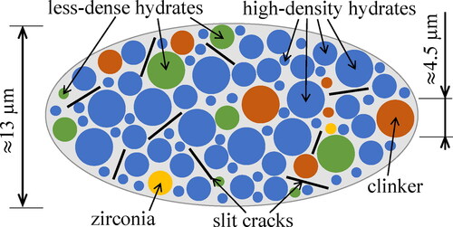
Figure 11. Probability density functions of (a) the bulk and (b) the shear moduli of the LDCR hydrates (red solid graphs) and of the HDCR hydrates (black solid graphs), as well as characteristic stiffness properties: equivalent stiffnesses (dash-dotted lines), mode values (dotted lines), and median values (solid lines).

Table 8. Results of the median-based piecewise uniform microelasticity model: strain concentration tensors components of the four types of solid constituents of Biodentine according to Eqs. (84)(84) $$A_{\mathit{vol},j}=\frac{1}{1+\frac{S_{\mathit{vol}}(k_j-k_{\mathit{bio}})}{k_{\mathit{bio}}}}\times {\left\{\sum _{i=1}^4\frac{f_i}{1+\frac{S_{\mathit{vol}}(k_i-k_{\mathit{bio}})}{k_{\mathit{bio}}}}\right\}}^{-1},$$(84) and (85)(85) $$A_{\mathit{dev},j}=\frac{1}{1+\frac{S_{\mathit{dev}}(g_j-g_{\mathit{bio}})}{g_{\mathit{bio}}}}\times {\{\sum _{i=1}^4\frac{f_i}{1+\frac{S_{\mathit{dev}}(g_i-g_{\mathit{bio}})}{g_{\mathit{bio}}}}+\frac{4\pi \omega }{3}{T}_{\mathit{dev}}\}}^{-1},$$(85) . The differences of the $A_{\mathit{vol},i},$ and $A_{\mathit{dev},i}$ values to the lognormal model are given in brackets.

Constituent of Biodentine	Strain concentration tensor components and deviations from lognormal microelasticity model
zirconia	$A_{\mathit{vol},1}=0.3036\hspace{1em}(-0.63\%)$	$A_{\mathit{dev},1}=0.2362\hspace{1em}(-0.43\%)$
clinker	$A_{\mathit{vol},2}=0.4250\hspace{1em}(-0.64\%)$	$A_{\mathit{dev},2}=0.3204\hspace{1em}(-0.38\%)$
HDCR hydrates	$A_{\mathit{vol},3}=1.0570\hspace{1em}(-0.18\%)$	$A_{\mathit{dev},3}=0.5250\hspace{1em}(-0.04\%)$
LDCR hydrates	$A_{\mathit{vol},4}=1.3068\hspace{1em}(+1.05\%)$	$A_{\mathit{dev},4}=0.6414\hspace{1em}(+0.22\%)$

Table 9. Results of the median-based piecewise uniform microelasticity model: stress concentration tensors components of the four types of solid constituents of Biodentine according to Eqs. (86)(86) $$B_{\mathit{vol},j}=\frac{k_j/k_{\mathit{bio}}}{1+\frac{S_{\mathit{vol}}(k_j-k_{\mathit{bio}})}{k_{\mathit{bio}}}}\times {\left\{\sum _{i=1}^4\frac{f_i}{1+\frac{S_{\mathit{vol}}(k_i-k_{\mathit{bio}})}{k_{\mathit{bio}}}}\right\}}^{-1},$$(86) and (87)(87) $$B_{\mathit{dev},j}=\frac{g_j/g_{\mathit{bio}}}{1+\frac{S_{\mathit{dev}}(g_j-g_{\mathit{bio}})}{g_{\mathit{bio}}}}\times {\{\sum _{i=1}^4\frac{f_i}{1+\frac{S_{\mathit{dev}}(g_i-g_{\mathit{bio}})}{g_{\mathit{bio}}}}+\frac{4\pi \omega }{3}{T}_{\mathit{dev}}\}}^{-1}.$$(87) . The differences of the $B_{\mathit{vol},i},$ and $B_{\mathit{dev},i}$ values to the lognormal model are given in brackets.

Constituent of Biodentine	Stress concentration tensor components and deviations from lognormal microelasticity model
zirconia	$B_{\mathit{vol},1}=1.3397\hspace{1em}(+0.16\%)$	$B_{\mathit{dev},1}=1.3397\hspace{1em}(+0.06\%)$
clinker	$B_{\mathit{vol},2}=1.2805\hspace{1em}(+0.18\%)$	$B_{\mathit{dev},2}=1.2805\hspace{1em}(+0.08\%)$
HDCR hydrates	$B_{\mathit{vol},3}=0.9722\hspace{1em}(+0.08\%)$	$B_{\mathit{dev},3}=0.9722\hspace{1em}(+0.01\%)$
LDCR hydrates	$B_{\mathit{vol},4}=0.8503\hspace{1em}(-0.87\%)$	$B_{\mathit{dev},4}=0.8503\hspace{1em}(-0.20\%)$

Figure A.12. Longitudinal and shear wave velocities sent at different frequencies through cylindrical samples of Biodentine, with 5 mm diameter and 10 mm height; the mean longitudinal wave velocity is equal to ${\overline{v}}_L=4.977$ km/s (upper data points cluster) and the mean shear wave velocity amounts to ${\overline{v}}_S=2.473$ km/s (lower data points cluster). The pink markers correspond to 50 kHz transducers central frequency, red to 500 kHz, cyan to 1 MHz, black to 2.25 MHz, green to 5 MHz, blue to 10 MHz, and yellow to 20 MHz transducers’ central frequency, after [3].

Table A.10. Ultrasonic shear wave transducers used for characterization of hardened Biodentine.

Frequency [MHz]	Shear transducer
2.25	V154-RM
5	V155-RM

P. Dohnalík, B.L. Pichler, L. Zelaya-Lainez, O. Lahayne, G. Richard, and C. Hellmich, Micromechanics of dental cement paste, J. Mech. Behav. Biomed. Mater., vol. 124, pp. 104863, 2021. DOI: 10.1016/j.jmbbm.2021.104863.

 PubMed Web of Science ®Google Scholar

R.J. Hussey, and J. Wilson, Advanced Technical Ceramics Directory and Databook, Springer Science & Business Media, Berlin, Heidelberg, 1998.

 Google Scholar

B. Pichler, and C. Hellmich, Upscaling quasi-brittle strength of cement paste and mortar: A multi-scale engineering mechanics model, Cement Concrete Res., vol. 41, no. 5, pp. 467–476, 2011. DOI: 10.1016/j.cemconres.2011.01.010.

 Web of Science ®Google Scholar