Figures & data
Figure 1. Example images of lung tissue examined in this study. (A) H&E image of biopsied lung tissue with pathologist-selected study areas outlined by yellow (low to moderate PM observed) and green boxes (high PM observed). (B) BSE image of the area marked with a black box in image A. The white box represents one of eleven frames that were analyzed to cover the area marked by the pathologist. (C) BSE image of the frame marked by the white box in image B shows inorganic PM (bright) in the lung tissue (dark). (D) Secondary electron image of the same frame shows the texture of the tissue.
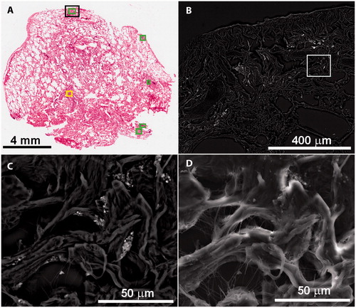
Figure 2. Examples of EDS spectra interpreted by specific mineral phases. (A) Secondary electron image shows tissue surrounding a particle cluster. (B) BSE image of same area with numbers marking locations of particles yielding the displayed spectra. Number designations touch the analyzed particles except 1, which refers to the bright circular grain. A total of 7 spectra were collected in this area.
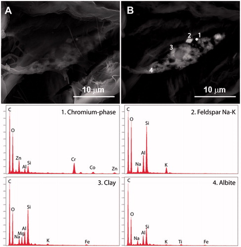
Figure 3. Example BSE images of in-situ aggregates of particles. (A) Polymineralic particle clusters. (B) Monomineralic cluster of calcium phosphate granules. (C) Monomineralic cluster of titanium dioxide. (D) Loose aggregate of mercury spheres.
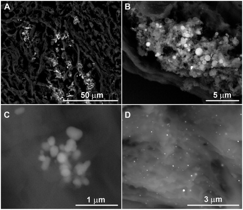
Figure 4. Pie diagrams summarizing the relative abundance of the eight major phase classes (silica, clay, feldspar, apatite, titanium dioxide, iron oxide, trace element-rich particles and steel) in samples for which in situ and digested tissue particles were identified and counted. For some samples, a duplicate of the filtered digested material was counted. The duplicate for sample 244 is an analysis of a second tissue slice. The numbers in parenthesis (#/#) display the ratio of the sum of all particles in the 8 major phase classes (silica, clay, feldspar, apatite, titanium dioxide, iron oxide, trace metals and steel) over the sum of all particles identified in that sample. The remainder of particles occurred at minor to trace amounts and did not fall into one of these 8 major phase classes. Data are compiled in Lowers et al. (Citation2016).
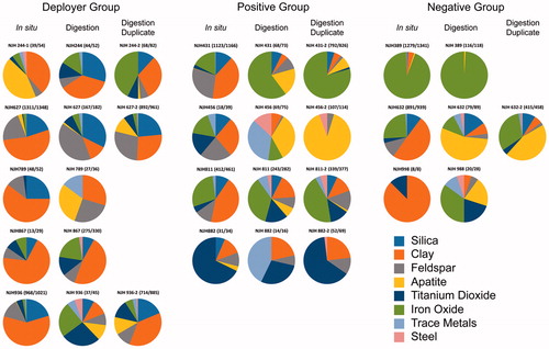
Table 1. Relative variance of the common phases at the frame (field of view), area (pathologist selected to focus analytical study), and subject levels calculated using linear mixed models on the relative abundances of the phases.
Table 2. Evaluation of the distribution of variance in tissue digestion results.
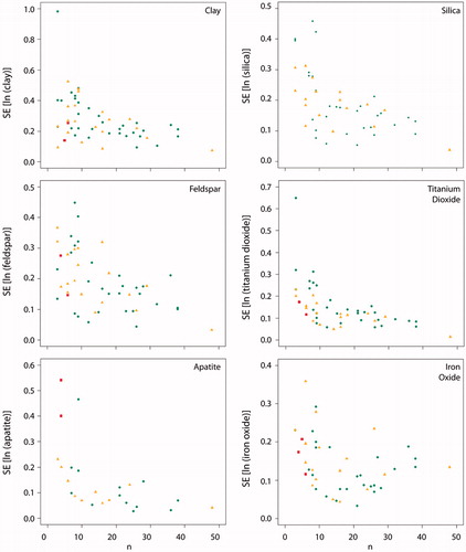
Table 3. Mean percentages of phases by method, with comparisons between methods using paired t-tests, based on n = 11 subjects.
Figure 5. Comparison of endogenic iron oxide aggregates. (A) Porous iron oxide observed during the in situ analysis commonly contained sodium (Na), phosphorus (P) and small amounts of sulfur (S) which may be part of the tissue or from tissue preparation. (B) Iron oxides observed after tissue digestion were less porous, contained less phosphorus, and had detectable chlorine (likely introduced from the bleach).
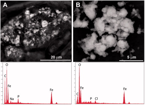
Figure 6. The bar charts summarize the mean relative abundance of the major phase classes for each of the pathologist defined tissue types containing high (green), moderate (yellow) and low (red) PM. The top chart includes all frames while the bottom chart is restricted to the frames that contained more than 5 particles.
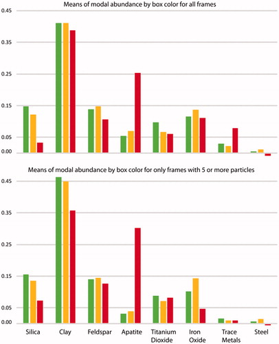
Figure 7. Plot of standard error (SE) versus the number of frames analyzed. Between 15–20 frames for silica, clay, feldspars, titanium dioxide and apatite was sufficient to achieve the minimal standard error. Iron oxide requires more frames to be counted to reduce the standard error. Colors of the data points indicate the pathologist area designation.