Mathematical model identifies effective P53 accumulation with target gene binding affinity in DNA damage response for cell fate decision

Figures & data

Figure 1. A mathematical p53 model identifies p53 terminal pulses. (a) Schematic representation of p53 regulatory network for our model. The numbers correspond to kinetic parameters in Table S2. The parameters k_f and k_r represent association and dissociation respectively between p53 mRNA and phosphorylated MDM2. (b) Concentration of total p53 level at various doxorubicin doses (Dox, from 0.01 to 1). (c) Maximal p53 levels under increasing Dox levels. (d) Time-averaged effective p53 integral (i.e. rate of effective p53 increase in units of μM) against increasing Dox levels was plotted. The end of the simulation is 40 h. (e) (Relative) local sensitivity coefficient of kinetic parameters for effective p53 integral (violet), p53 pulse height (red) and period (green). The most sensitive parameters were marked. The local sensitivity is in units of 1. (f) Correlation between sensitivity measures was shown. R denotes Spearman correlation coefficient. ‘Ep53ʹ denotes effective p53 integral.

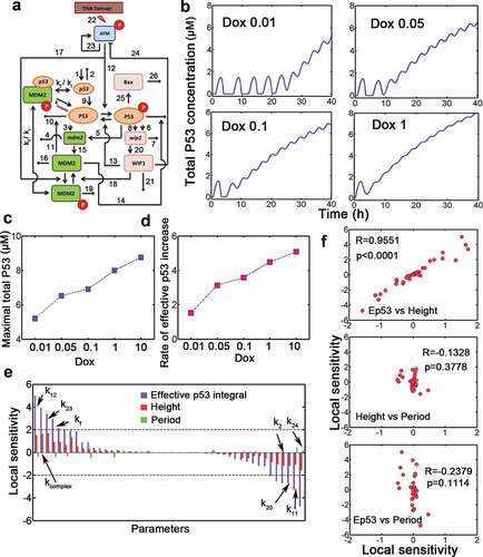
Figure 2. Dynamic features of dual-phase p53 under stimulation by different Dox dosage. (a) Selected total p53 trajectories when Dox = 0.01, 0.1 and 10. Note that the unit of ‘p53 levels’ in stochastic simulation is 1. (b) Fraction of terminal pulses at different Dox levels. (c) Comparison of effective p53 integral between survival and apoptotic cells. The unit for effective p53 integral during stochastic simulation is ‘min’ thereafter. (d-e) Lifespan (d) and terminal pulse height (e) treated by relatively low levels (0.01, 0.05 and 0.1) of Dox. Data were represented as mean±SD. (f) Effective p53 integral of apoptotic cells under different Dox levels. (g) Pulse height (top) and duration (bottom) for cells with Dox = 0.01, 0.05 and 0.1.

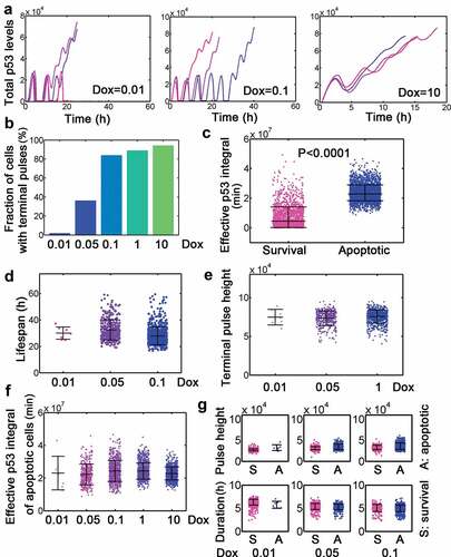
Figure 3. Simulation of effect Nutlin-3 treatment. (a) Representative traces of p53 treated with Dox = 0.1 combined with Nutlin-3 added immediately or at 6 and 16 h, following Dox treatment. To simulated the effect of Nutlin-3 treatment, k₁₁ and k₁₄ were simultaneously lowed by 5 fold. (b-e) Lifespan (b), terminal pulse height (c), total p53 integral (d) and effective p53 integral in apoptotic cells (e) for 500 simulations with nutlin-3 addministration immediately or at 6 and 16 h (Dox = 0.1), respectively. ANOVA was used to detect the statistical significance. **: P < 0.01.

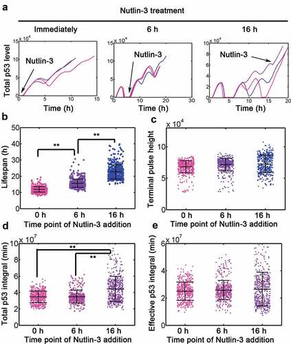
Figure 4. Gene expression specificity by p53 binding affinity and target gene stability. (a) Relative fold change of target gene expression under 0.1 and 0.01 Dox treatment with varying binding affinity (K_m in μM, equivalent to k₁₁ in Table S1) and target gene degradation rates (δ, min⁻¹). Arrows represent exemplified situations in (B). (b) Stochastic simulations of target gene expression with varying transcription factor binding affinity and target gene stability. The mean trajectories (solid) for control (Dox = 0.00005, red), 0.01 (blue) and 0.1 (black) Dox were shown. Shaded areas represent 95% confidence intervals. (c) The integral of putative downstream effector (i.e. p53 target gene) under control, 0.01 and 0.1 Dox treatment was depicted with δ = 0.0001 (min⁻¹). N = 50 cases of stochastic simulations in (B) were shown. K_m values (from left to right: 0.01, 0.07, 0.15 and 0.3 μM) were displayed on top. (d) Effective p53 integral under 0.01 and 0.1 Dox treatment, respectively. Mann-Whitney test was used.

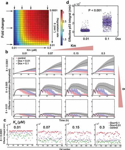
Figure 5. P53 dynamics decompose into distinct signaling classes. (a) Time-resolved analysis of p53 dynamics for varying stimulus levels as indicated (Dox = 0.01–10). 20 representative cases were shown as well as the population median (red). (b) P53 dynamics were clustered into 5 signaling classes according to their time-resolved data. The population median values were shown (red). (c) Distributions of signaling classes depending on Dox levels. (D-E) Silhouette plots of cells sorted according to signaling classes (d) and Dox levels (e). Positive silhouette scores indicate that P53 dynamics are more similar to the own group, whereas negative scores indicate that the trajectory is closer to any of the other groups. (f) The lifespan distribution of cells treated with different Dox levels (top) or dynamic clusters (top). Note that if cell survived during the whole simulation period (60 h), the lifespan was recorded as 60 h. (g) Effective p53 integral for cells with varying Dox (top) and different clusters (bottom).

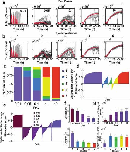
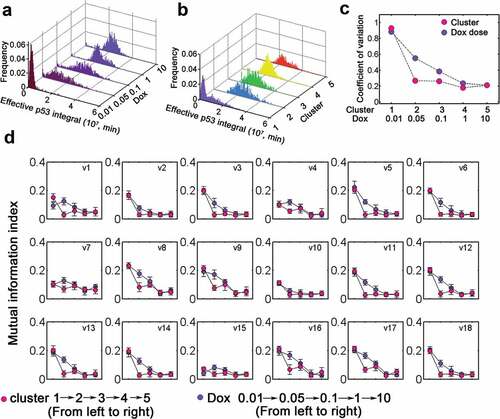
Figure 6. Classification into dynamic clusters produces switch-like transition. (a) Distribution of effective p53 integral for varying Dox levels (0.01–10). (b) Distribution of effective p53 integral for five dynamic clusters. (c) The coefficient of variation for cells stimulated with various Dox (violet) or in distinct clusters (rose carmine). (d) Mutual information index with increasing Dox (violet) and different clusters (rose carmine). The details for kinetic processes (v₁-v₁₈) were listed in Table S3.