Safety assessment of automated vehicles: how to determine whether we have collected enough field data?

Figures & data

Figure 1. The true pdfs $g\left(\cdot \right)$ (black solid line) and $h(\cdot )$ (gray dashed line) that are used to illustrate the quantification of the completeness.

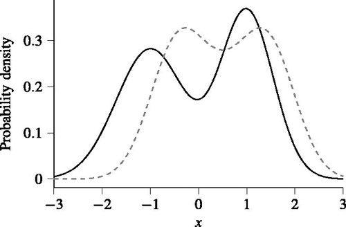
Figure 2. The bandwidths of $\widehat{f}(\cdot ;n)$ (black dashed line), $\widehat{g}(\cdot ;n)$ (gray solid line), and $\widehat{h}(\cdot ;n)$ (gray dotted line) for the example with artificial data. The bandwidths are computed using leave-one-out cross-validation for different numbers of samples $n.$

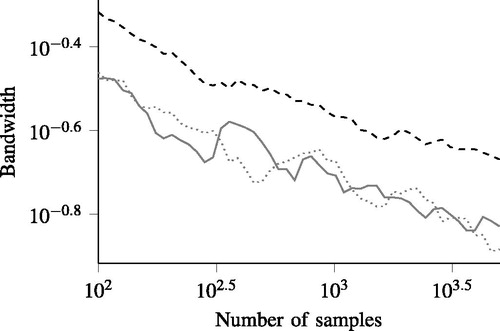
Figure 3. The real MISEs (black lines) of the example of with the artificial data, approximated using Eq. (13)(13) $${\mathrm{MISE}}_f\left(n\right)\approx \frac{1}{m}{\sum }_{j=1}^m{\int }_{{\mathbb{R}}^d}{\left(f\left(x\right)-{\widehat{f}}_j\left(x;n\right)\right)}^2\mathrm{ }\mathrm{d}x,$$(13) , and the measures that are used to quantify the completeness (gray lines). The solid lines show the result of estimating a bivariate pdf, so here Eq. (8)(8) $$J_f\left(n\right)=\frac{h^4}{4}{\sigma }_K^4{\int }_{{\mathbb{R}}^d}{\left({\nabla }^2\widehat{f}\left(x;n\right)\right)}^2\mathrm{ }\mathrm{d}x+\frac{{\mu }_K}{n{h}^d}.$$(8) is used to quantify the completeness. The dashed lines show the result of estimating 2 univariate pdfs and combining them according to Eq. (10)(10) $$f\left(x\right)=g\left(y\right)h\left(z\right),$$(10) to create a bivariate pdf, so Eq. (12)(12) $$J_f\left(n\right)=J_g\left(n\right){\int }_{{\mathbb{R}}^{d_z}}\widehat{h}{\left(z;n\right)}^2\mathrm{ }\mathrm{d}z+J_h\left(n\right){\int }_{{\mathbb{R}}^{d_y}}\widehat{g}{\left(y;n\right)}^2\mathrm{ }\mathrm{d}y+J_g\left(n\right)\cdot J_h\left(n\right).$$(12) is used to quantify the completeness. The gray areas show the interval $\left[\mu -3\sigma ,\mu +3\sigma \right],$ where $\mu$ and $\sigma$ denote the mean and standard deviation, respectively, of the measures of Eqs. (8)(8) $$J_f\left(n\right)=\frac{h^4}{4}{\sigma }_K^4{\int }_{{\mathbb{R}}^d}{\left({\nabla }^2\widehat{f}\left(x;n\right)\right)}^2\mathrm{ }\mathrm{d}x+\frac{{\mu }_K}{n{h}^d}.$$(8) and (12)(12) $$J_f\left(n\right)=J_g\left(n\right){\int }_{{\mathbb{R}}^{d_z}}\widehat{h}{\left(z;n\right)}^2\mathrm{ }\mathrm{d}z+J_h\left(n\right){\int }_{{\mathbb{R}}^{d_y}}\widehat{g}{\left(y;n\right)}^2\mathrm{ }\mathrm{d}y+J_g\left(n\right)\cdot J_h\left(n\right).$$(12) when repeating the experiment 200 times.

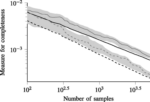
Figure 4. Histogram of the data used for the example with the real data.

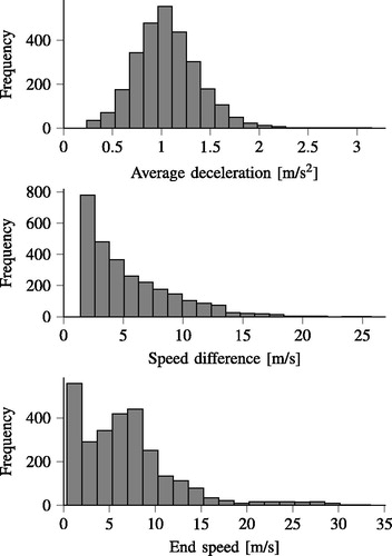
Figure 5. The bandwidths of $\widehat{f}(\cdot ;n)$ (black dashed line), $\widehat{g}(\cdot ;n)$ (gray solid line), and $\widehat{h}(\cdot ;n)$ (gray dotted line) for the example of with the real data. The bandwidths are computed using leave-one-out cross-validation for different numbers of samples $n.$

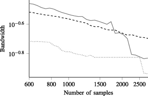
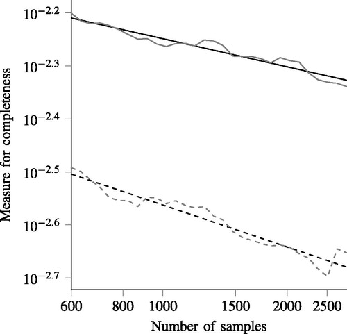
Figure 6. The measures of completeness for the example with the real data with the assumption that all 3 parameters depend on each other (gray solid line) and with the assumption that the first parameter—that is, the average deceleration—does not depend on the other 2 parameters (gray dashed line). The corresponding black lines represent the least squares logarithmic fits given by Eqs. (14)(14) $$0.019\cdot n^{-0.18},$$(14) and (15)(15) $$0.017\cdot n^{-0.26},$$(15) .