Optimization of Characteristics Polymer Composite Reinforced Kenaf and Jute Fiber Using Taguchi-Response Surface Methodology Approach

Figures & data

Figure 1. Kenaf fiber.

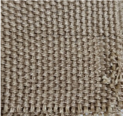
Figure 2. Jute fiber.

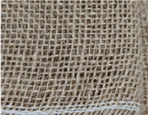
Table 1. Bisphenol-A epoxy resin property.

Properties	Unit	Value
Viscosity	MPa	13.000 ± 2.000
Epoxy number	%	22.7 ± 0.6
Epoxy equivalent	g/equiv	189 ± 5
Epoxy value	Equiv/100 g	0.53 ± 0.01
Total chlorine content	%	<0.2
Hydrolyzable chlorine content	%	<0.05
Color according to the Gardner scale	-	<1
Density at 25°C	g/cm^3	1.17 ± 0.01
Refractive index at 25°C	-	1.572 ± 0.003
Volatile content at 3 h, 140°C	%	<0.2
Vapor pressure at 80°C	mbar	<0.1
Flashpoint, according to DIN 51,584	°C	>250

Table 2. CMNFR fabrication parameters.

Control factor	Level 1	Level 2	Level 3
A	4%	6%	8%
B	80°C	100°C	120°C
C	JF	KF	KF-JF

Table 3. Design matrix of orthogonal array L₂₇³ for the experimental runs.

Trial number	A	B	C
1	1	1	2
2	1	1	2
3	1	1	2
4	1	2	1
5	1	2	1
6	1	2	1
7	1	3	3
8	1	3	3
9	1	3	3
10	2	1	1
11	2	1	1
12	2	1	1
13	2	2	3
14	2	2	3
15	2	2	3
16	2	3	2
17	2	3	2
18	2	3	2
19	3	1	3
20	3	1	3
21	3	1	3
22	3	2	2
23	3	2	2
24	3	2	2
25	3	3	1
26	3	3	1
27	3	3	1

Table 4. Mechanical strength of CMNFR.

Trial number	Uncoded value of factor			Impact Strength (J/mm^2)	Flexural Strength (MPa)
	A	B	C
1	1	1	2	2.6 × 10^−2	6.5 × 10^1
2	1	1	2	2.4 × 10^−2	3.4 × 10^1
3	1	1	2	2.3 × 10^−2	3.9 × 10^1
4	1	2	1	1.2 × 10^−2	6.7 × 10^1
5	1	2	1	1.2 × 10^−2	7.1 × 10^1
6	1	2	1	9.6 × 10^−3	7.3 × 10^1
7	1	3	3	1.4 × 10-^2	7.1 × 10^1
8	1	3	3	1.4 × 10^−2	7.5 × 10^1
9	1	3	3	1.4 × 10^−2	7.4 × 10^1
10	2	1	1	8.9 × 10^−3	5.7 × 10^1
11	2	1	1	1.1 × 10^−2	6.3 × 10^1
12	2	1	1	9.9 × 10^−3	5.3 × 10^1
13	2	2	3	1.1 × 10^−2	6.8 × 10^1
14	2	2	3	1.2 × 10^−2	6.8 × 10^1
15	2	2	3	1.3 × 10^−2	7.0 × 10^1
16	2	3	2	1.7 × 10-^2	9.1 × 10^1
17	2	3	2	1.9 × 10^−2	9.4 × 10^1
18	2	3	2	1.6 × 10^−2	9.1 × 10^1
19	3	1	3	1.3 × 10^−2	7.2 × 10^1
20	3	1	3	1.2 × 10^−2	7.3 × 10^1
21	3	1	3	1.4 × 10^−2	7.2 × 10^1
22	3	2	2	1.9 × 10^−2	7.2 × 10^1
23	3	2	2	1.8 × 10^−2	7.3 × 10^1
24	3	2	2	1.7 × 10^−2	7.0 × 10^1
25	3	3	1	5.8 × 10^−3	6.8 × 10^1
26	3	3	1	8.2 × 10^−3	6.4 × 10^1
27	3	3	1	5.6 × 10^−3	6.6 × 10^1

Figure 3. Vacuum infusion laminates steps.

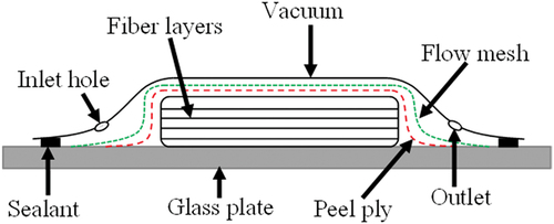
Figure 4. VARI process.

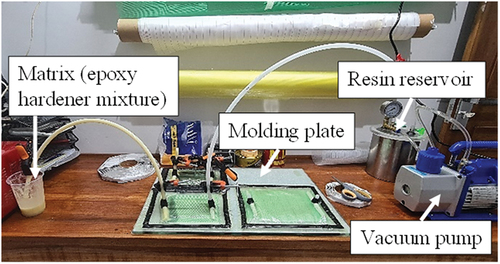
Figure 5. Drying process.

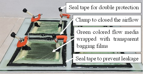
Figure 6. Specimen release.

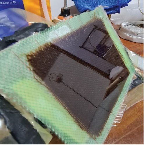
Figure 7. Specimen cutting results.

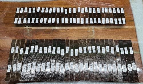
Figure 8. A schematic diagram of this research.

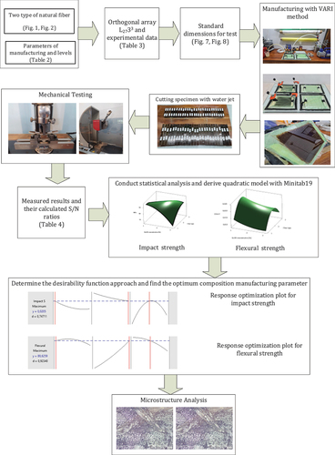
Table 5. ANOVA analysis of impact strength and flexural strength.

Control Factor	Level 1	Level 2	Level 3	Delta	Rank
	Impact strength
SN ratio for impact strength (dB)
(A)	−36.15	−37.96	−38.97	2.82	2
(B)	−36.75	−37.51	−38.82	2.07	3
(C)	−41.05	−34.24	−37.79	6.81	1
Means (μm)
(A)	0.016537	0.0131	0.01242	0.004117	2
(B)	0.015714	0.013729	0.012614	0.003099	3
(C)	0.009349	0.019749	0.012958	0.0104	1
	Flexural strength
SN ratio for flexural strength (dB)
(A)	35.52	37.05	36.90	1.52	2
(B)	34.91	36.91	37.65	2.74	1
(C)	36.14	36.26	37.06	0.92	3
Means (μm)
(A)	63.14	72.74	70.06	9.60	2
(B)	58.72	70.11	77.13	18.41	1
(C)	64.59	69.98	71.37	6.78	3

Figure 9. Plots of mean and SN ratios of composite material strength: (a) impact; (b) flexural.

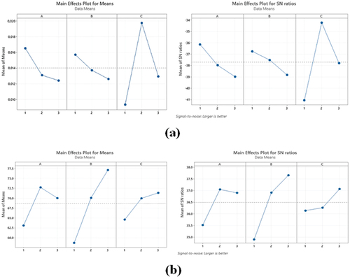
Table 6. CI calculated confidence interval.

Response	N	95% CI for μ
Impact strength	27	(0.012; 0.016)
Flexural strength	27	(63.55; 73.75)

Table 7. Comparisons of results of the experimental and Taguchi predicted value.

Response	Experimental result	Calculated value	Confidence interval (CI)	Difference Strengthexp-Strengthcal	Optimization
Impact strength	Strengthexp = 0.026	Strengthcal = 0.024	CIStrength = 0.014	0.002	0.002 < 0.014 Successful
Flexural strength	Strengthexp = 90.6	Strengthcal = 83.9	CIStrength = 68.65	6.7	6.7 < 68.65 Successful

Table 8. ANOVA analysis of impact strength and flexural strength.

Source	DF	Seq. SS	Contribution	Adj. SS	Adj. MS	F-Value	P-Value
ANOVA for impact strength
Model	8	6.34 × 10^−4	95.94%	6.34 × 10^−4	7.90 × 10^−5	53.22	0
Linear	3	1.78 × 10^−4	26.94%	1.50 × 10^−4	5.00 × 10^−5	33.58	0
A	1	7.60 × 10−5	11.54%	7.60 × 10−5	7.60 × 10−5	51.20	0
B	1	4.30 × 10−5	6.54%	2.20 × 10−5	2.20 × 10−5	14.70	1 × 10−3
C	1	5.90 × 10−5	8.86%	3.40 × 10−5	3.40 × 10−5	22.62	0
Square	3	4.56 × 10^−4	68.94%	3.44 × 10^−4	1.15 × 10^−4	76.94	0
A*A	1	1.10 × 10^−5	1.72%	1.10 × 10^−5	1.10 × 10^−5	7.65	1.30 × 10^−2
B*B	1	1 × 10^−6	0.17%	1 × 10^−6	1.00 × 10^−6	0.55	4.70 × 10^−1
C*C	1	4.43 × 10^−4	67.04%	3.22 × 10^−4	3.22 × 10^−4	216.42	0
2-Way Interaction	2	0	0.07%	0	0	0,15	8.62 × 10^−1
A*B	1	0	0.07%	0	0	0,21	6,55 × 10−1
A*C	1	0	0.00%	0	0	0	9,72 × 10^−1
Error	18	2.70 × 10^−5	4.06%	2.7 × 10^−5	1 × 10^−6
Total	26	6.61 × 10^−4	100%
ANOVA for flexural strength
Model	8	3.67 × 10^3	85.16%	3.67 × 10^3	4.59 × 10^2	12.91	0
Linear	3	1.95 × 10^3	45.16%	2.25 × 10^3	7.52 × 10^2	21.14	0
A	1	2.15 × 102	4.99%	2.15 × 102	2.15 × 102	6.06	2.40 × 10−2
B	1	1.53 × 103	35.37%	1.90 × 103	1.90 × 103	53.38	0
C	1	2.07 × 10^2	4.79%	3.80 × 10^−1	3.80 × 10^−1	0.01	9.19 × 10^−1
Square	3	2.79 × 10^2	6.47%	4.34 × 10^2	1.45 × 10^2	4.07	2.30 × 10^−2
A*A	1	2.26 × 10^2	5.25%	2.26 × 10^2	2.26 × 10^2	6.37	2.10 × 10^−2
B*B	1	2.86 × 10^1	0.66%	4.41 × 10^1	4.41 × 10^1	1.24	2.80 × 10^−1
C*C	1	2.40 × 10^1	0.56%	1.41 × 10^2	1.41 × 10^2	3.96	6.20 × 10^−2
2-Way Interaction	2	1.45 × 10^3	33.53%	1.45 × 10^3	7.23 × 10^2	20.34	0
A*B	1	9.38 × 102	21.74%	2.32 × 102	2.32 × 102	6.54	2 × 10−2
A*C	1	5.08 × 10^2	11.79%	5.08 × 10^2	5.08 × 10^2	14.30	1 × 10^−3
Error	18	6.40 × 10^2	14.84%	6.40 × 10^2	3.56 × 10^1
Total	26	4.31 × 10^3	100%

Figure 10. 3D RSM plot of the strength of natural fiber composite materials: (a) NaOH vs. post-curing temperature for impact strength; (b) NaOH vs. post-curing temperature for flexural strength.

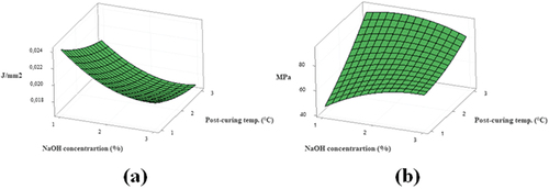
Figure 11. Plots of response optimization (D= composite desirability; d= individual desirability; High = highest value parameter; Cur= optimal current value of control parameter; Low = lowest value parameter, y= response parameter, A= NaOH concentration; B= post-curing temperature; C= fiber type).

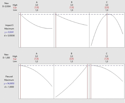
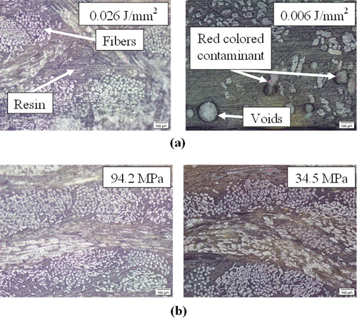
Figure 12. Micro photos of composite specimens; (a) impact test specimen, (b) flexural test specimen.