Effects of Physical and Mechanical Properties of Coir Fiber and Reinforced Epoxy Composites Treated with Acetic Anhydride and Alkali

Figures & data

Table 1. Details of literature review with kind of fiber and treatment method.

No.	Author	Fiber	Treatment method	Purpose	Research field
1	Gonzalez-Lopez et al (2019a)	coir fiber	maleic anhydride, methyl vinyl ether-alt-maleic anhydride	To improve the compatibility of coir fibers with poly (lactic acid) by two different surface treatments of fibers	PLA based bio-composites, injection molding
2	Ban et al. (2020)	bamboo fiber	glycerol treatment, aluminate ester treatment, silane treatment	To solve the issue of poor interface adhesion between bamboo fibers and cement matrix	natural-fiber-reinforced cement-based materials
3	Siakeng et al. (2020)	coir fiber, pineapple leaf fiber	alkali-treated	To deal with the incorporation of different ratios of fibers in polylactic acid hybrid composites	sustainable and degradable hybrid composites
4	Asumani and Paskaramoorthy (2020)	kenaf fiber	alkali-alone treatment and combined alkali-silane treatment	To investigate two fiber treatments on the fatigue and impact strengths of kenaf fiber reinforced polypropylene composites	natural fiber-based polymer composites
5	Hashim et al. (2017)	kenaf fiber	alkali treatment	To explore alkali treatment on kenaf fiber physical properties under various conditions	environment friendly reinforcement material
6	Kumar and Das (2017)	nettle fiber	alkali treatment	To improve tensile strength, elongation-at-break and initial modulus of nettle fibers with alkali treatment	textile-reinforced polymer matrix composites
7	El Boustani et al. (2017)	flax fiber, kraft pulp fiber	acetylation treatment	To investigate acetylation treatment of fibers on the impregnation and tensile properties of composites.	flax fiber/epoxy, high-performance green composites
8	Silva, Maia, and Mulinari (2021)	Sugarcane bagasse	acetylation treatment	To investigate the acetylation’s influence on sugarcane bagasse fiber’s structure and properties	natural fiber composites
9	Senthilraja et al (2020)	palm fiber	acetylation treatment	To eliminate the swelling effect of the palm fiber composite by Acetylation	natural fiber reinforced polymer composites
10	Gieparda et al. (2021)	flax fiber	silanization, plasma modification	To investigate the effectiveness of the combination of chemical and physical methods of natural fibers’ modification.	natural-fiber-based materials

Figure 1. Getting coir fiber (a) and flow chart of composite production (b).

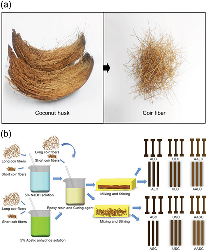
Figure 2. (a) The TGA curves of UCF (black)、AACF (red) and ACF (blue) under optimal conditions. (b) the DTG curves of UCF (black)、AACF (red) and ACF (blue) under optimal conditions.

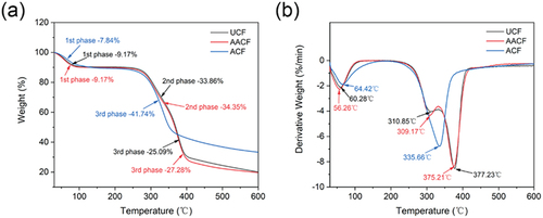
Figure 3. FTIR spectra of UCF (black)、AACF (red) and ACF (blue) under optimal conditions.

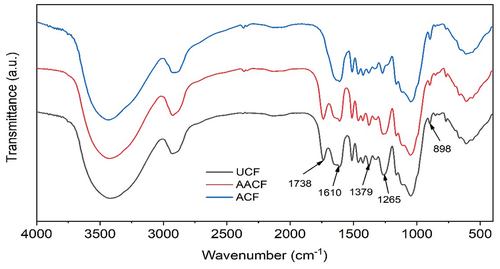
Table 2. Peak value of change in FTIR spectrum.

Wavenumbers (cm^−1)			Functional groups
UCF	AACF	ACF
1738	1738	̸	C=O
1610	1610	1610	C=C
1379	1379	1379	C-H
1265	1265	1265	C-O
898	898	898	C-H

Figure 4. Diameter (a), tensile strength (b), and morphology (c) of different types of coir fibers.

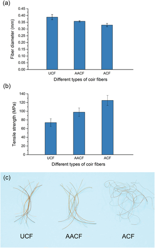
Figure 5. Tukey test for coir fiber tensile strength.

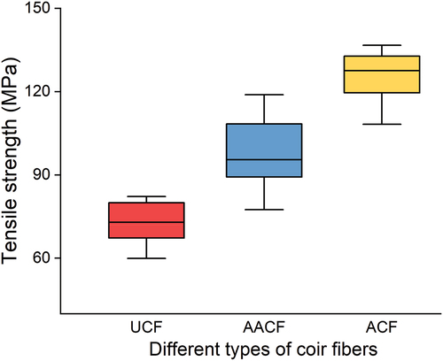
Table 3. ANOVA for coir fiber tensile strength.

Source	Sum of squares	df	Mean square	F-value	p-value
Intergroup	6895.57	2	3447.79	21.82	<0.001**	highly significant
Intragroup	1896.03	12	158.01

**p-value <0.01 (highly significant, **).

Figure 6. Microscopic SEM images of the surface of UCF (a), a part of the surface of UCF (b), surface of AACF (c), a part of the surface of AACF (d), surface of ACF (e), and a part of the surface of ACF (f).

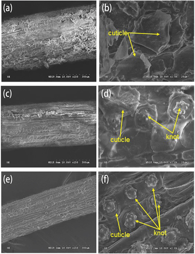
Figure 7. The tensile stress–strain curves of PEB (a), ULC (b), USC (c), AALC (d), AASC (e), ALC (f), and ASC (g).

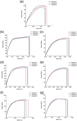
Figure 8. Tensile strength of different specimens (a), Tukey test for different specimens (b).

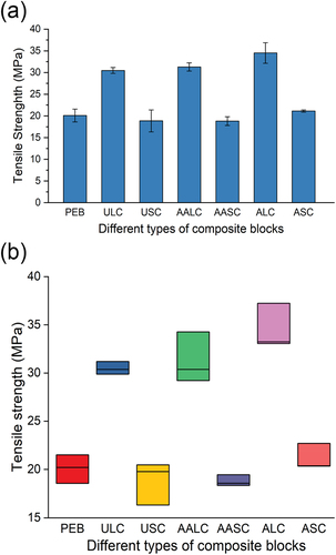
Table 4. ANOVA for composite tensile strength.

Source	Sum of squares	df	Mean square	F-value	p-value
Intergroup	825.77	6	137.63	43.20	<0.001**	highly significant
Intragroup	44.60	14	3.19

**p-value <0.01 (highly significant, **).

Figure 9. The flexural stress–strain curves of PEB (a), ULC (b), USC (c), AALC (d), AASC (e), ALC (f), and ASC (g).

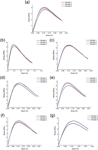
Figure 10. Flexural strength of different specimens (a), Tukey test for different specimens (b).

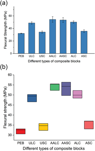
Table 5. ANOVA for composite flexural strength.

Source	Sum of squares	df	Mean square	F-value	p-value
Intergroup	1689.99	6	281.67	61.06	<0.001**	Highly significant
Intragroup	64.58	14	4.61

**p-value <0.01 (highly significant, **).

Figure 11. Microscopic SEM images of ULC fracture surface (a), USC fracture surface (b), AALC fracture surface (c), AASC fracture surface (d), ALC fracture surface (e), and ASC fracture surface (f).

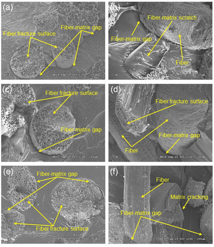
Figure 12. Percentage increase in weight of the composites at room temperature (a), Tukey test for different specimens (b).

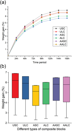
Table 6. ANOVA for composite hygroscopicity.

Source	Sum of squares	df	Mean square	F-value	p-value
Composite	4.38	5	0.88	77.98	<0.001**	Highly significant
Time	71.63	6	11.94	1062.05	<0.001**
Error	0.34	30	0.01

**p-value <0.01 (highly significant, **).

Gonzalez-Lopez, M. E., A. A. Perez-Fonseca, R. Manriquez-Gonzalez, M. Arellano, D. Rodrigue, and J. R. Robledo-Ortiz. 2019a. “Effect of Surface Treatment on the Physical and Mechanical Properties of Injection Molded Poly (Lactic Acid)-Coir Fiber Biocomposites.” Polymer Composites 40 (6): 2132–2141. https://doi.org/10.1002/pc.24997.

 Web of Science ®Google Scholar

Ban, Y., W. Zhi, M. E. Fei, W. D. Liu, D. M. Yu, T. F. Fu, and R. H. Qiu. 2020. “Preparation and Performance of Cement Mortar Reinforced by Modified Bamboo Fibers.” Polymers 12 (11): 2650. https://doi.org/10.3390/polym12112650.

 PubMed Web of Science ®Google Scholar

Siakeng, R., M. Jawaid, M. R. Saba, N. Sanjay, H. Siengchin, S. Fouad, and H. Fouad. 2020. “Alkali Treated Coir/Pineapple Leaf Fibres Reinforced PLA Hybrid Composites: Evaluation of Mechanical, Morphological, Thermal and Physical Properties.” Express Polymer Letters 14 (8): 717–730. https://doi.org/10.3144/expresspolymlett.2020.59.

 Web of Science ®Google Scholar

Asumani, O., and R. Paskaramoorthy. 2020. “Fatigue and Impact Strengths of Kenaf Fibre Reinforced Polypropylene Composites: Effects of Fibre Treatments.” Advanced Composite Materials 30 (2): 103–24. https://doi.org/10.1080/09243046.2020.1733308.

 Web of Science ®Google Scholar

Hashim, M. Y., A. M. Amin, O. M. F. Marwah, M. H. Othman, M. R. M. Yunus, and N. C. Huat. 2017. “The Effect of Alkali Treatment Under Various Conditions on Physical Properties of Kenaf Fiber.” International Conference on Materials Physics and Mechanics 914:12030. https://doi.org/10.1088/1742-6596/914/1/012030.

 Google Scholar

Kumar, N., and D. Das. 2017. “Alkali Treatment on Nettle Fibers: Part I: Investigation of Chemical, Structural, Physical, and Mechanical Characteristics of Alkali-Treated Nettle Fibers.” The Journal of the Textile Institute 108 (8): 1461–1467. https://doi.org/10.1080/00405000.2016.1257346.

 Web of Science ®Google Scholar

El Boustani, M., G. Lebrun, F. Brouillette, and A. Belfkira. 2017. “Effect of a Solvent-Free Acetylation Treatment on Reinforcements Permeability and Tensile Behaviour of Flax/Epoxy and Flax/Wood Fibre/Epoxy Composites.” The Canadian Journal of Chemical Engineering 95 (6): 1082–1092. https://doi.org/10.1002/cjce.22777.

 Web of Science ®Google Scholar

Silva, N. G. S., T. F. Maia, and D. R. Mulinari. 2021. “Effect of Acetylation with Perchloric Acid as Catalyst in Sugarcane Bagasse Waste.” Journal of Natural Fibers 19 (13): 5050–5064. https://doi.org/10.1080/15440478.2021.1875352.

 Web of Science ®Google Scholar

Senthilraja, R, Sarala, R, Antony, A. G, and Seshadhri. 2020 Effect of acetylation technique on mechanical behavior and durability of palm fibre vinyl-ester composites Materials Today: Proceedings 21 634–637. https://doi.org/10.1016/j.matpr.2019.06.729.

 Google Scholar

Gieparda, W., S. Rojewski, and W. Rozanska. 2021. “Effectiveness of Silanization and Plasma Treatment in the Improvement of Selected Flax Fibers’ Properties.” Materials 14 (13): 3564. https://doi.org/10.3390/ma14133564.

 PubMed Web of Science ®Google Scholar