Investigation of the occurrence of binder material on airborne respirable mineral wool fibers

Figures & data

Table 1. Collected samples and analysis techniques used in this study.

	SW-A GW-A	SW-B GW-B	SW-C	GW-C	SW-D
Sample type	Wool product	Air-collected fiber	Air-collected fiber	Air-collected fiber	Air-collected fiber
Airborne fiber collection method		2	3	3	3
Number of samples	SW: 1; GW: 1	SW: 5; GW: 6	1	3	3
Filter		Polycarbonate 25 mm	Polycarbonate 25 mm	Polycarbonate 25 mm	Polycarbonate 25 mm
Airflow [l/min]		2	13	22	32
Analysis	SEM	SEM EDXS	SEM EDXS	SEM EDXS	SEM EDXS
Figure	1 and 2	4 and 5	6	7	8

Figure 1. Scanning electron microscope (SEM) image (BSE 5 kV) of the stone wool product used in the present study: (a) sample SW-A ROCKWOOL A-Batts density of 30 kg/m³ and organic content 2.0 wt. % of solid matter; (b) sample SW-A—light grey is the fiber (A) and dark areas on the fibers are binder (B); (c) and (d) sample SW-A where the binder material was removed by heat treatment of the sample at 590 °C for 20 min.

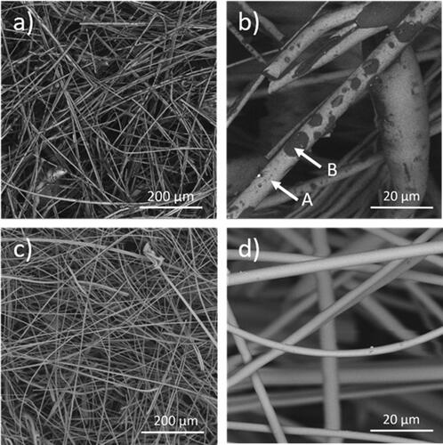
Figure 2. Scanning electron microscope (SEM) image (BSE 5 kV) of the glass wool product used in the present study: (a) sample GW-A – 37 ISOVER Basic Formstykker density of 18 kg/m³ and organic content 6.4 wt. % of solid matter; (b) sample GW-A—light grey is the fiber (A) and dark areas on the fibers are binder (B); (c) and (d) sample GW-A where the binder material was removed by heat treatment of the sample at 450 °C for 120 min.

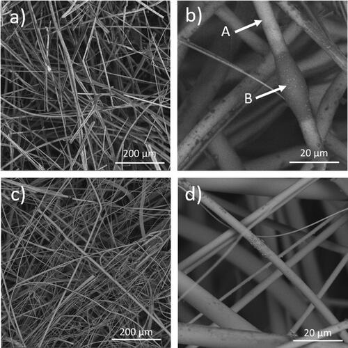
Figure 3. Fiber diameter distribution of (a) sample SW-A (product type is ROCKWOOL A-Batts density of 30 kg/m³) and (b) sample GW-A (product type is 37 ISOVER 37 Basic Formstykker density of 18 kg/m³).

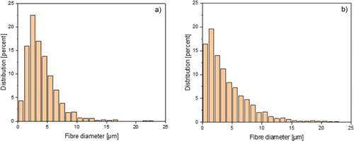
Figure 4. SEM image (BSE 5 kV) of sample SW-B, fibers collected on the filter using Method 2 (airflow rate 2 l/min): (a) collected fibers with random diameter distribution; (b)–(c) two fibers with diameter < 3 µm with dark areas of the organic material; (d) EDXS spectra showing a marked carbon peak and decrease in other elements levels corresponding to the dark spot position. The EDXS data was obtained from the same location as in (c).

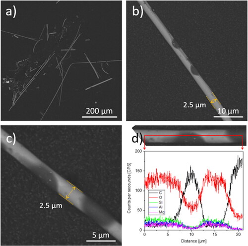
Figure 5. SEM image (BSE 5 kV) of sample GW-B, fibers collected on the filter using Method 2 (airflow rate 2 l/min): (a) collected fibers with random diameter distribution; (b)–(c) two fibers with diameter < 3 µm with dark areas of the organic material; (d) EDXS spectra showing a marked carbon peak and decrease in other elements levels corresponding to the dark spot position. The EDXS data was obtained from the same location as in (c).

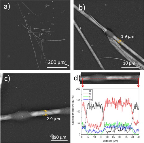
Figure 6. SEM image (BSE 5 kV) of sample SW-C, fibers collected on the filter using Method 3 (airflow rate of 13 l/min): (a) collected fibers with random diameter distribution; (b)–(c) two fibers with diameter < 3 µm with dark areas of the organic material; (d) EDXS spectra showing a marked carbon peak and decrease in other elements levels corresponding to the dark spot position. The EDXS data was obtained from the same location as in (c).

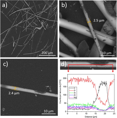
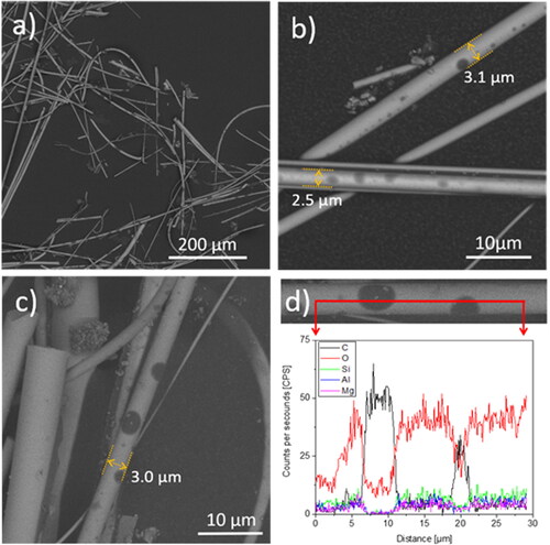
Figure 7. SEM image (BSE 5 kV) of sample GW-C, fibers collected on the filter using Method 3 (airflow rate of 22 l/min): (a) collected fibers with random diameter distribution; (b)–(c) two fibers with diameter < 3 µm with dark areas of the organic material; (d) EDXS spectra showing a marked carbon peak and decrease in other elements levels corresponding to the dark spot position. The EDXS data was obtained from the same location as in (c).

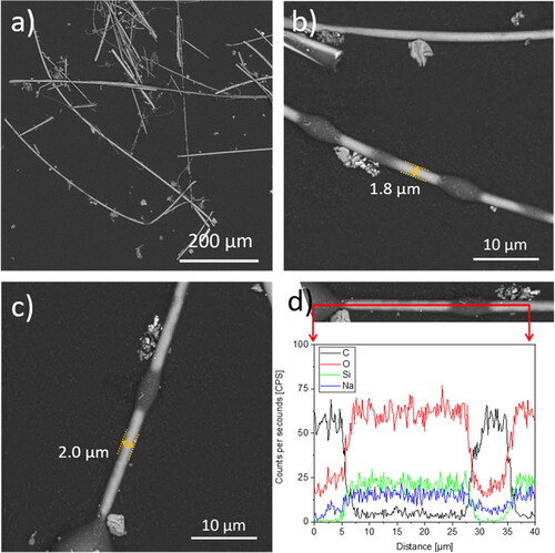
Figure 8. SEM image (BSE 5 kV) of sample SW-D, fibers collected on the filter using Method 3 (airflow rate of 32 l/min): (a) collected fibers with random diameter distribution; (b)–(c) two fibers with diameter < 3 µm with dark areas of the organic material; (d) EDXS spectra showing a marked carbon peak and decrease in other elements levels corresponding to the dark spot position. The EDXS data was obtained from the same location as in (c).

Data availability

The data that support the findings of this study are available from the corresponding author, MS, upon reasonable request.