Revealing representative day-types in transport networks using traffic data clustering

Figures & data

Table 1. Summary table of network-wide day clustering.

Data Type	Internal	Clustering	Classification	Similarity	Centroid	Dimensionality reduction	Train set [days]	Test set [days]	Prediction model	Paper
speed	TWCV, TCD	k-means, spectral, DBSCAN	ED	MI	Consensus	–	35	1	centroid-based	Lopez et al. (2017)
speed, flow	TWCV, TCD	k-means, spectral	ED	MI, AMI,CS	Consensus, historical-mean	–	127	30	centroid-based	Cebecauer et al. (2019)
speed	TWCV, TCD	k-means	ED	MI	Consensus, shape-based, historical-mean	PCA	34	35 × 1	centroid-based	Krishnakumari et al. (2020)
speed	TWCV, TCD, SC	k-means, GMM	ED	MI	Consensus	PCA	167	56	centroid-based	Chiabaut and Faitout (2021)
speed, flow	TWCV	Two-step(calendar, agglomerative)	–	Ward	–	–	118	–	–	W. Weijermars and Van Berkum (2005)
flow	–	Two-step (calendar, gravitational)	calendar & maximal vertical difference	=classi.	Historical-mean	–	42	10	trivial, moving average, exponential smoothing	Wild (1997)
flow	SC, DB, CH	spectral, affinity propagation	–	ED	–	PCA, SVD	290	–	–	Yang et al. (2017)
flow	–	calendar	mean ED	=classi.	–	–	730	52	exponential smoothing, linear curve fitting	Chrobok et al. (2004)
flow	–	calendar	calendar, RF	–	–	–	361	359	LSTM, RF	Toqué et al.,(2017)
flow	TWCV	calendar, k-mean	calendar, ED	ED	Historical-mean	PCA, SVD	212	54	centroid-based, Persistence method, ARIMA, VAR	Ferranti (2020)
speed, flow	calendar	calendar	calendar	–	–	–	21	7	Multivariete nonparametric regression	Clark (2003)

Table uses followint abbrevations: Silhouette Score (SC), Davies-Bouldin index (DB), Euclidean Distance (ED), Gaussian Mixture Model (GMM), Mutual Information (MI), Adjusted Mutual Information (AMI), Cosine Similarity (CS), Calinski-Harabasz(CH), Random forest (RF) Long-Short Term Memory (LSTM), Autoregressive Integrated Moving Average method (ARIMA), Vector Autoregression method (VAR).35x1 for Test dataset in Krishnakumari et al. (2020) refers to leave-one-out strategy for all 35 days.

Figure 1. Overview of the methodological framework for revealing the representative set of day-types Y with internal and external evaluation, including dimensionality reduction, day clustering. External evaluation process is highlighted.

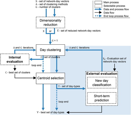
Table 2. Notation

Notation	Description
d	Index of day
N	Number of days or network-day vectors
$N_T$	Set of training days
$N_C$	Set of calibration days
$N_E$	Set of evaluation days
j	Index of time interval
J	Number of time intervals
i	Index of observation entity
I	Number of observation entities in the network
X	matrix with network-day vectors
$X_T$	matrix of network-day vectors in set $N_T$
$X_C$	matrix of network-day vectors in set $N_C$
$X_E$	matrix of network-day vectors in set $N_E$
$x_d$	Network-day vector of day d
$v_{ij}^{x_d}$	Observation on network-day vector $x_d$ of day d at time interval j and observation entity i.
$v_m^{x_d}$	Observation at the m dimension of the network-day vector $x_d$ of day d.
M	Number of dimensions, $M=I\times J$
G	Number of day clusters
C	Set of G clusters $C=\{C_1,C_2,\dots ,C_G\}$
$y_g$	Centroid of the cluster g (day-type)
$y_{(}g,i,j)$	Value of centroid g for observation entity i and interval j
Y	Set of clusters’ centroids (day-types)
R	Maximal number of past intervals to be consider in classification and local smoothing
f	Index of future time interval
F	Set of future time intervals to be considered in prediction and calibration

Table 3. Sets of calendar-based clustering categories.

Abbreviation	Full name	Cluster’s categories description
dow	day-of-week	Monday, Tuesday, Wednesday, Thursday, Friday, Saturday, Sunday
wkd	weekend/weekday	Monday – Friday, Saturday – Sunday
hol	holiday	No holiday, Public holiday, School holiday, De-facto holiday

Figure 2. Case study of motorway control system sensors of Stockholm, Sweden active at least one day 2017-2018. The sensors with complete data in case study period are highlighted. (a) Complete network of active sensors. (b) Area around the city center. (c) Zoom-in illustration of the sensor density.

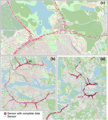
Table 4. Internal evaluation indices for calendar-based clusterings.

Clustering C	|C|	Non-empty clusters
${\text{cal}}_{\text{dow}}$	7	7
${\text{cal}}_{\text{wkd}\times \text{hol}}$	8	7
${\text{cal}}_{\text{dow}\times \text{hol}}$	28	26

Figure 3. Calendar visualization of calendar-based clusterings for year 2017. White cells are days with missing data.

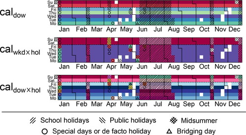
Figure 4. Calendar visualization of data-driven clustering methods clustered on original dataset $X_T.$ White cells are days with missing data.

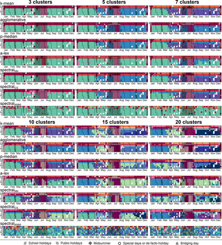
Figure 5. Day-type centroids for p-median and a-lex with 10 clusters. (a) Calendar visualization (b) Aggregated network-wide day-time profiles. (c,d) Space-time matrices of flows across all sensors in the network and all considered time intervals. (c) for p-median and (d) for a-lex.

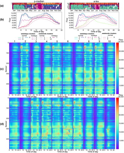
Figure 6. Total within-cluster variance (TWCV) as a function of the number of clusters across clustering methods. (a) is the original dataset $X_T$ and (b) the reduced dataset ${\overline{X}}_T.$

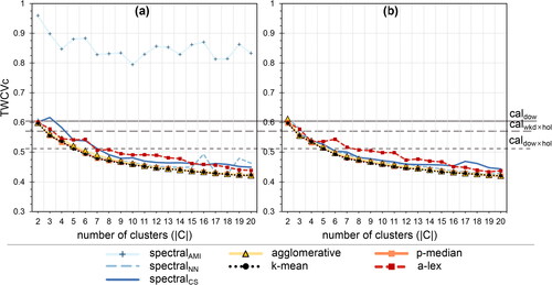
Figure 7. Total cluster dissimilarity (TCD) as a function of the number of clusters across clustering methods. (a) is the original dataset $X_T$ and (b) the reduced dataset ${\overline{X}}_T.$

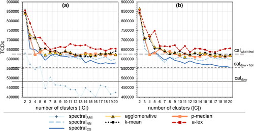
Figure 8. Silhouette score (SC) as a function of the number of clusters across clustering methods. (a) is the original dataset $X_T$ and (b) the reduced dataset ${\overline{X}}_T.$

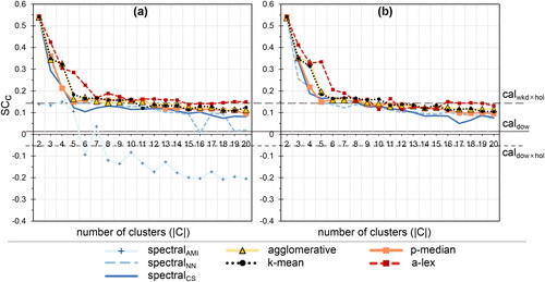
Figure 9. Davies-Bouldin (DB) index as a function of the number of clusters across clustering methods. (a) is the original dataset $X_T$ and (b) the reduced dataset ${\overline{X}}_T.$

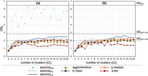
Figure 10. Short-term prediction performance external validation index as a function of the number of clusters across clustering methods. (a) is the original dataset $X_T$ and (b) the reduced dataset ${\overline{X}}_T.$

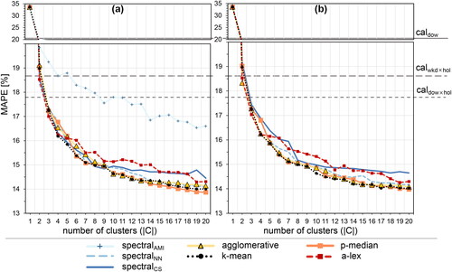
Figure 11. Exponential smoothing short-term prediction performance external validation index of the clustering C as a function of the number of clusters. (a) is the original dataset $X_T$ and (b) the reduced dataset ${\overline{X}}_T.$

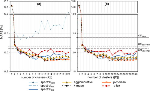
Table 5. Best performing number of clusters according to considered internal indices per clustering method. The clusterings considered as best and reasonable are highlighted in bold.

Clustering method	TWCV& TCD	SC	DB	all in consideration
${\text{spectral}}_{\text{NN}}$	5,7	7	7	7
${\text{spectral}}_{\text{CS}}$	4,8	8	6,8	8
agglomerative	4,7	4,6	6,11	4,6
k-means	4,6	4, 7	6, 10	4,6
p-median	6,10	7,11	6, 11	6,11
a-lex	5,11	5, 8	4, 11	5,11

Table 6. Total computational time for clustering methods to run 19 clusterings with 2-20 clusters.

	Computational time [s]
Clustering method	Original dataset $X_T$	Reduced dataset ${\overline{X}}_T$
${\text{spectral}}_{\text{AMI}}$	42,135.54	–
${\text{spectral}}_{\text{NN}}$	12.52	8.74
${\text{spectral}}_{\text{CS}}$	239.87	271.16
Agglomerative	85.00	4.92
k-means	202.50	7.80
p-median	3,203.00	292.95
a-lex	4,130.93	1391.82

Lopez, C., Leclercq, L., Krishnakumari, P., Chiabaut, N. and Lint, H. (2017). Revealing the day-to-day regularity of urban congestion patterns with 3d speed maps. Scientific Reports, 7(1), 14029. https://doi.org/10.1038/s41598-017-14237-8

 PubMedGoogle Scholar

Cebecauer, M., Gundlegård, D., Jenelius, E. and Burghout, W. (2019). 3d speed maps and mean observations vectors for short-term urban traffic prediction. In Transportation Research Board Annual Meeting (TRB) (pp. 1–20).

 Google Scholar

Krishnakumari, P., Cats, O. and van Lint, H. (2020). A compact and scalable representation of network traffic dynamics using shapes and its applications. Transportation Research Part C: Emerging Technologies, 121, 102850. https://doi.org/10.1016/j.trc.2020.102850

 Web of Science ®Google Scholar

Chiabaut, N. and Faitout, R. (2021). Traffic congestion and travel time prediction based on historical congestion maps and identification of consensual days. Transportation Research Part C: Emerging Technologies, 124, 102920. https://doi.org/10.1016/j.trc.2020.102920

 Web of Science ®Google Scholar

Weijermars, W. and Van Berkum, E. (2005). Analyzing highway flow patterns using cluster analysis. In Proceedings. 2005 IEEE Intelligent Transportation Systems, 2005 (pp. 308–313). https://doi.org/10.1109/ITSC.2005.1520157

 Google Scholar

Wild, D. (1997). Short-term forecasting based on a transformation and classification of traffic volume time series. International Journal of Forecasting, 13(1), 63–72. https://doi.org/10.1016/S0169-2070(96)00701-7

 Google Scholar

Yang, C., Yan, F. and Xu, X. (2017). Daily metro origin-destination pattern recognition using dimensionality reduction and clustering methods. In 2017 IEEE 20th International Conference on Intelligent Transportation Systems (ITSC) (pp. 548–553). https://doi.org/10.1109/ITSC.2017.8317899

 Google Scholar

Chrobok, R., Kaumann, O., Wahle, J. and Schreckenberg, M. (2004). Different methods of traffic forecast based on real data. European Journal of Operational Research, 155(3), 558–568. https://doi.org/10.1016/j.ejor.2003.08.005

 Web of Science ®Google Scholar

Toqué, F., Khouadjia, M., Come, E., Trepanier, M. and Oukhellou, L. (2017). Short & long term forecasting of multimodal transport passenger flows with machine learning methods. In 2017 IEEE 20th International Conference on Intelligent Transportation Systems (ITSC) (pp. 560–566). https://doi.org/10.1109/ITSC.2017.8317939

 Google Scholar

Ferranti, F. (2020). Public transport origin-destination matrices: Pattern recognition and short-term prediction. KTH Royal institute of technology.

 Google Scholar

Clark, S. (2003). Traffic prediction using multivariate nonparametric regression. Journal of transportation engineering, 129(2), 161–168. https://doi.org/10.1061/(ASCE)0733-947X(2003)129:2(161)

 Web of Science ®Google Scholar