Figures & data
FIGURE 1. Mechanism of rhythmic contractions of smooth muscle, driven by pacemaker activity from ICC. This diagram represents the membrane potential of a smooth muscle cell, which is alternating between hyperpolarised and hypopolarised states; this pattern is referred to as slow waves. The function of slow waves is to change membrane potential from a state of low open probability (hyperpolarised) for voltage-dependent calcium ion (Ca2+) channels to open (−80 to −55 mV), to a hypopolarised state, where there is elevated probability of Ca2+ channel opening (−40 to −25 mV). Where the membrane potential is above the threshold for action potentials, voltage-gated Ca2+ channels open, and allow Ca2+ influx, indicated by the red arrows.Citation17 This transient Ca2+ influx then initiates smooth muscle contraction. This is the mechanism by which slow waves drive rhythmic contractions of smooth muscle.
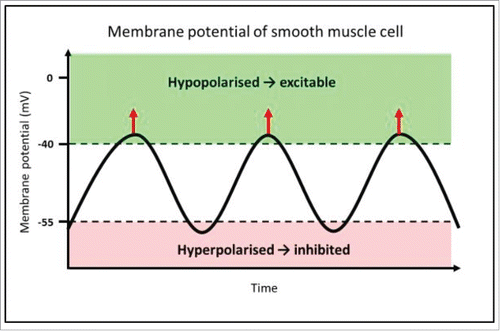
FIGURE 2. A diagrammatic representation of the relationship between neurons, ICC and motor patterns. The parasympathetic nervous system, a subgroup of the autonomic nervous system, provides input to the enteric nervous system, promoting digestion and defecation.Citation24,25 The enteric nervous system is known to control peristalsis.Citation11 However, the link between the enteric nervous system and ICC is debated, and this relationship is what we aim to test in this study. ICC transmit pacemaker activity to smooth muscle cells, causing slow wave changes in membrane potential.Citation13-16 This then drives rhythmic contractions of smooth muscle cells, and it is these contractions which we observe in the organ bath. Anticholinergic drugs are known to have negative input to both the parasympathetic nervous system and the enteric nervous system, by blocking cholinergic neurotransmission.Citation47,48 By treating the intestine with these drugs and measuring the rhythmic contractions driven by ICC, we examine whether there is a link between enteric neurons and ICC.
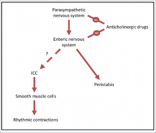
FIGURE 3. Fast Fourier Transform for conversion of signal from time to frequency domain. On the left is the signal in time domain of length N-1 samples, whereby the lower-case x[ ] represent signal value at every time point. Then, this signal is processed by forward DFT to give the frequency spectrum, whereby the amplitude X[ ] can be computed. Here, X[ ] has 2 components, whereby Re X[ ], being the real values, represents the amplitudes of the cosine wave, and Im X[ ], being the imaginary values, represents the amplitudes of sine wave, with each having a length of N/2+1. These are collectively referred to as X[ ], which sum up to a length of N-1.
![FIGURE 3. Fast Fourier Transform for conversion of signal from time to frequency domain. On the left is the signal in time domain of length N-1 samples, whereby the lower-case x[ ] represent signal value at every time point. Then, this signal is processed by forward DFT to give the frequency spectrum, whereby the amplitude X[ ] can be computed. Here, X[ ] has 2 components, whereby Re X[ ], being the real values, represents the amplitudes of the cosine wave, and Im X[ ], being the imaginary values, represents the amplitudes of sine wave, with each having a length of N/2+1. These are collectively referred to as X[ ], which sum up to a length of N-1.](/cms/asset/e96fa19d-46bb-4dff-967e-e4ae8c7f1f58/kogg_a_1295904_f0003_c.gif)
FIGURE 4. An example of the output of Fast Fourier Transform. (A) This graph records fluctuations in diameter of a transverse slice of intestine over time. The red and blue arrows represent the highest and lowest diameter respectively of that particular video analysis. Owing to the intrinsic width of the intestine, fluctuations cannot be about the zero mark, but rather around the length-dependent variable diameter of the intestine. (B) The frequency spectrum plot shows the most salient frequency – that is, the frequency with the highest amplitude, to choose the predominant frequency and amplitude. This allows elimination of other signals that contribute to ‘noise’ in the graph of diameter change over time, which ideally should be sinusoidal in shape. This method is used to eliminate human error in counting the number of contractions over time and using an average, which is used currently in the literature. As well as this, it allows more detailed information about the amplitude of contractions, which is difficult to measure, and as yet has not been studied in detail in gastrointestinal motility experiments in the literature.
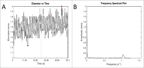
FIGURE 5. Gastrointestinal Motility Monitor and organ bath setup. (A) The GIMM is a complete system required to measure GI non segmentation contractions in small animal models such as mice and guinea pigs. The organ bath setup is represented as follows: A pump circulates the warmed, aerated Krebs solution into the organ bath, where the dissected intestine sits. The intestine is pinned down in the organ bath, to allow a camera to record the organ motility. (B) For each trial, first the organ is allowed to equilibrate in the Krebs solution for 10 minutes. Next, a 5 minute video of the untreated organ is recorded and used as the internal control. After that, the drug was added at a therapeutic plasma concentration, allowed to equilibrate in the solution for 5 minutes, and then recorded for 5 minutes. A supratherapeutic concentration was then added, allowed to equilibrate for 5 minutes, and then recorded for 5 minutes.
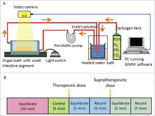
FIGURE 6. Analysis of video recordings. (A) An image of the organ with no contrast. The analysis program finds this difficult to analyze;(B) An image of the organ with full contrast; the black organ is easily measured by the analysis program; (C) An example of the image without covering up calibration markings and sides of the organ bath – the program in this case spuriously records calibration markers as part of the organ.
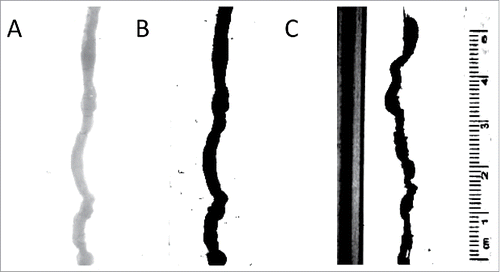
FIGURE 7. Spatiotemporal maps for data analysis of an untreated mouse small intestine. Using the motor analysis function, spatiotemporal motor maps of the mouse small intestine were generated and analyzed. (A) Two-dimensional spatiotemporal map: The software from the GIMM system includes the output of a spatiotemporal map recording distance, time and diameter measurements. This spatiotemporal map is used as the input for our analysis program. Distance is the x-axis, time is the y-axis and the diameter changes are recorded using shades from black to white. (B) Three-dimensional intensity map of the 3 variables, namely, distance, diameter and time, in the form of a 3D spatiotemporal plot. The area highlighted in red indicates the cross-section of the organ chosen, which we can see oscillates in diameter as contractions occur. This change in diameter over time is analyzed to measure frequency and amplitude of contractions. Diameters are represented in grayscale so that contractions were shown in black, relaxations are shown in white and the intermediate gray regions represent diameters from 0.7 mm to 5 mm as shown in the scale indicated by the red arrow.
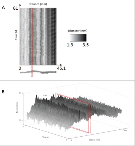
FIGURE 8. Signal processing of the time domain signals based on the following procedures: 1) Averaging of all signals in the Distance (mm) axis (represented by gray) into a single green signal (with its peaks and toughs highlighted by red and blue triangles respectively); 2) Perform moving average of the signal of interest to produce a smoothed signal that has its sharp peaks reduced; 3) Convert signal from time to frequency domain by applying Fast Fourier Transform (with dominant peaks highlighted by red dots); and 4) Deduce the dominant pairs of amplitude and frequency by identifying the dominating peaks of the frequency spectrum graph to give the stem plot (with the ends of every stem highlighted by a red dot). Note that A, B, and C denotes the increment of the inspection window in the moving average filter that leads to increased smoothing of the signal of interest. This corresponds to a reduction in the number of stems for the frequency spectrum stem plot.
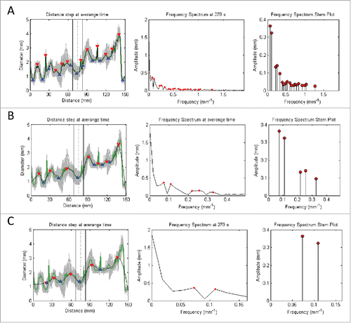
FIGURE 9. Frequency and amplitude of gastrointestinal motility over 1 hour for organs that are: (A) Untreated baseline; (B) Treated with benztropine; and (C) Treated with promethazine. The 3 different conditions can be quantified based on their respective frequency spectrums.
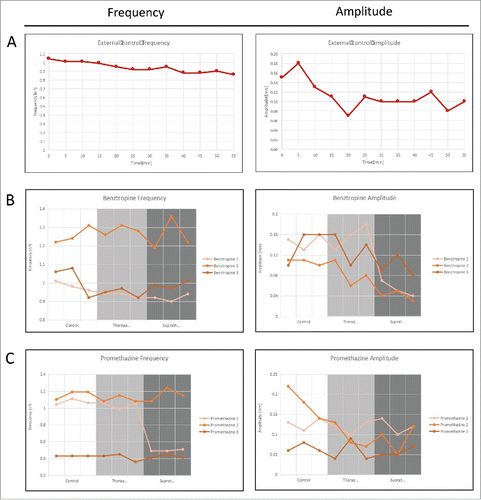
TABLE 1. Benztropine results.
TABLE 2. Promethazine results.
TABLE 3. Individual results whereby significant results have been highlighted in bold.
TABLE 4. Summary of significant changes in individual experiments.
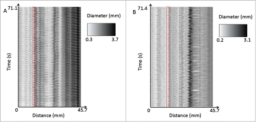
FIGURE 10. A comparison of the spatiotemporal maps of one of the benztropine internal controls (A) and its paired benztropine supratherapeutic trial (B). The control shows more regular contractions throughout the entire length of the organ, whereas the supratherapeutic drug trial shows more irregular and less well-defined contractions. This can be seen for example in the areas highlighted in red, where in the control, the variation in diameter is regular and the amplitude is large, where in comparison the therapeutic trial shows more irregular, lower amplitude contractions.