Figures & data
Table 1. Interfaces in ribosomal assemblies.
Table 2. Comparison with binary complexes.
Table 3. Amino acid and Nucleotide composition.
Figure 1. Area-based propensities of (a) aminoacid residues and (b) nucleotides at PP, PR and RR interfaces in ribosomal assemblies.
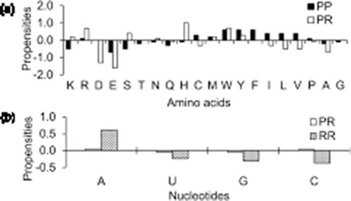
Table 4. Chemical composition of the interfaces.
Table 5. Hydrogen bond composition.
Figure 2. Propensities of stacking interactions: (a) residues at PP and PR interfaces and (b) nucleotides at PR and RR interfaces.
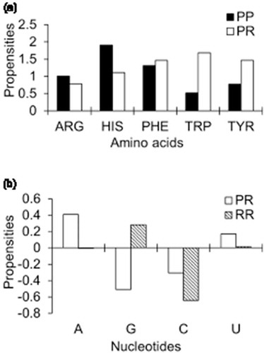
Figure 3. Frequency distributions of a number of interacting partners of large and small subunits r-proteins as well as RNAs, both in prokaryotes and eukaryotes.
Figure 4. The macromolecular interaction networks of (a) 70S and (b) 80S ribosomal assemblies. Protein and RNA molecules are represented by the node of the graph and their interactions by the edges. The edges of the network are divided based on the interface area B into (i) solid (B > 4000 Å2), (ii) broken (2000 Å2 < B > 4000 Å2) and (iii) grey (B < 2000 Å2).
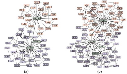
Table 6. Classification of r-proteins.
Figure 5. The box plot showing the distributions of different features of pairwise interfaces for three classes of r-proteins: (a) interface area B and (b) structural and physicochemical features in (i) early (ii) intermediate and (iii) late binders. The box plot (whisker diagram) is a standardized way of displaying the distribution of data based on the five-number summary: minimum, first quartile, median, third quartile, and maximum. In the simplest box plot the central rectangle spans the first quartile to the third quartile (the interquartile range or IQR). A segment inside the rectangle shows the median and ‘whiskers’ above and below the box show the locations of the minimum and maximum.
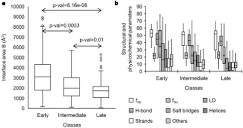
Figure 6. Confusion matrix predicting the classification of r-proteins as (i) early (ii) intermediate and (iii) late binders using RF. Scale represents the percentage of instances.