Tutorial: Color Rendering and Its Applications in Lighting

Figures & data

Fig. 1 Stages in the perception of a red strawberry.

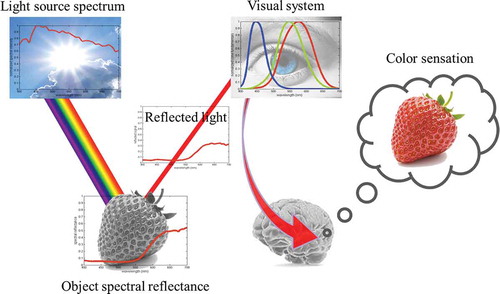
Fig. 2 Spectral power distributions (SPDs) for some of the phases of the reference illuminants used in the computation of CRI. All SPDs are in relative units, normalized to have a value of 1.0 at 560 nm.

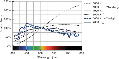
Fig. 3 Spectral reflectance functions for a green apple and strawberry.

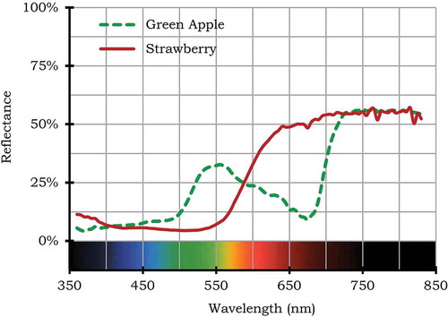
Fig. 4 Net relative spectral sensitivity of the human eye’s three cone cell types.

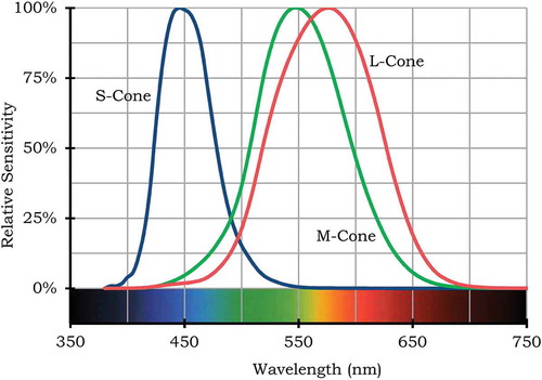
Fig. 5 The 1931 CIE 2° standard observer, including the , and color matching functions (CMFs), sometimes also called the XYZ CMFs. For historical background, see MacAdam [1970].

Fig. 6 CIE 1931 chromaticity diagram illustrating the location of the spectrum locus, purple boundary, blackbody locus, and several lines of constant CCT. Note that the background colors are more symbolic than literal because color appearance depends on several additional factors that are not included in this chart, such as luminance, background, and context.

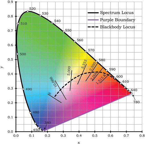
Fig. 7 Three SPDs that have the same chromaticity, which means that they are metameric. Because chromaticity is identical (0.4369, 0.4041), the CCT is also identical (3000 K in this example), yet these sources will render objects very differently. The CRI values are 34 for the three-LED mixture, 94 for the four-LED mixture, and 100 for the blackbody radiator.

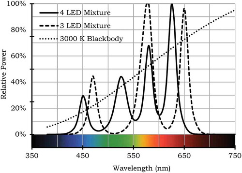
Fig. 8 Influence of adaptation on color appearance. Left: Two scenes, one at noon (top) and the other at sunset (bottom), as they would appear without chromatic adaptation. Right: The same two scenes as viewed with chromatic adaptation. Note that chromatic adaptation corrects, to a degree, for the slight bluish and yellowish color cast present in the top and bottom left images, respectively.

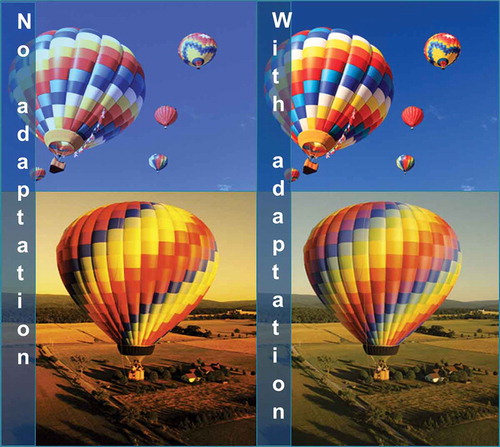
Fig. 9 Cases “A” (left) and “B” (right), as described in the text, illustrating the same room illuminated with two different light sources that provide the same illuminance and have the same chromaticity but different spectral power distributions.

Fig. 10 Spatial illumination pattern (right) and its graphical depiction (left) showing illuminance (E) vs. position measured along the dotted line (x).

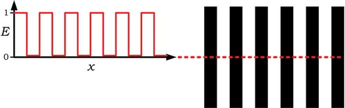
Fig. 11 Spatial reflectance pattern (right) and its graphical depiction (left) showing reflectance (R) vs. position measured along the dotted line (x).

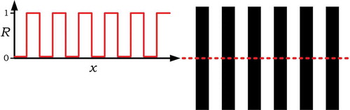
Fig. 12 Overlapping the illumination pattern of Fig. 10 onto the reflectance pattern of Fig. 11 and plotting the intensity pattern of the reflected light, which is the mathematical product of illuminance, E, and reflectance, R, thus denoted as ER. In this example, because of the relative spacing, there is no position that simultaneously has non-zero illumination and non-zero reflectance, so in this case no light reflects anywhere.

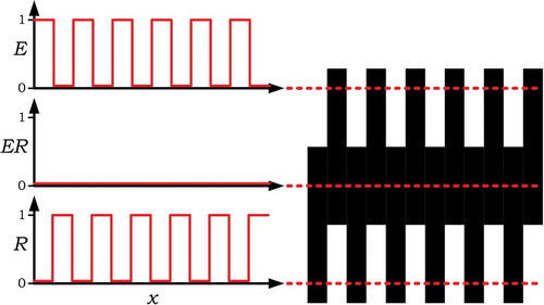
Fig. 13 The same situation as in Fig. 12, except that the reflectance pattern has a slightly increased spacing, so that toward the right portion of the pattern regions of non-zero illumination overlap with regions of non-zero reflectance, so that there is considerable reflected light.

Fig. 14 The same situation as in Fig. 13, except that the illuminance and reflectance patterns are much finer. The same overall variation in reflected intensity is apparent.

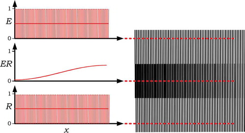
Fig. 15 In analogy to Fig. 13, this shows an illuminant spectral power distribution that varies with wavelength, illuminating a surface whose spectral reflectance function also varies with wavelength. In this case the product ER is the spectral power distribution of the reflected light, often called the color stimulus function. ER displays, effectively, a moiré pattern in the wavelength domain.

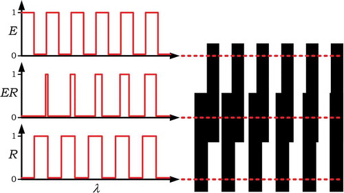
Fig. 16 Eight color samples used to calculate R_a and the first eight R_i values.

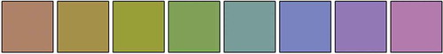
Fig. 17 Six color samples used to calculate R_i values 9 to 14.

Fig. 18 Schematic of the CRI calculation.

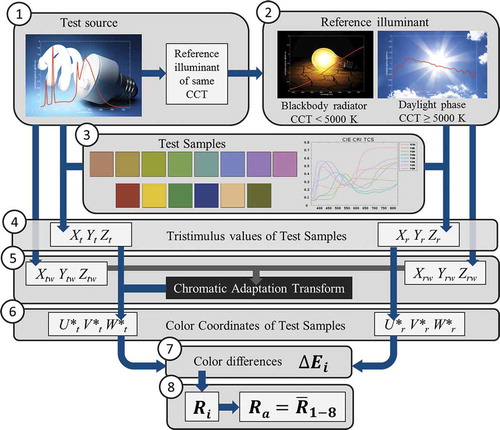
Fig. 19 The left box was illuminated with 100 CRI light (from two 60 W, 2750 K incandescent lamps) and the matching objects at right were illuminated with 80 CRI light (from two 13 W, 2750 K CFL lamps). They were photographed simultaneously in a single digital camera image. Compared to the left, at right the red pepper, strawberries, and tomatoes appeared less red, the wood looked slightly greenish, and the purple petunia and violet lobelia petals appeared blue. Other objects had smaller color shifts.

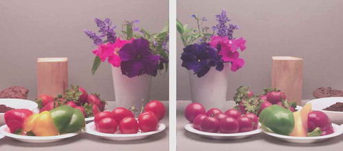
Fig. 20 Example of two fairly jagged SPDs that both have the same fairly high R_a value of 93. The SPD shown with a solid line is for a source with chromaticity of (0.3386, 0.3509) and CCT of 5250 K. The SPD shown with a dashed line is for a source with chromaticity of (0.3804, 0.3767) and CCT of 4000 K.

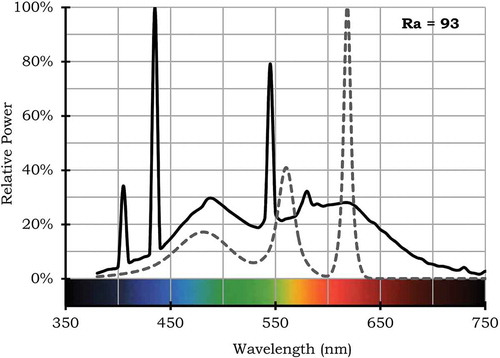
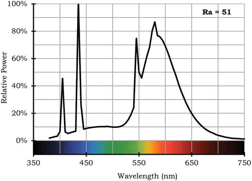
Fig. 21 Example of a fairly complete SPD that has a fairly low R_a value of 51.

APPENDIX A: TERMS TABLE A.1 Definition of key concepts that support an understanding of color rendering

Concept	Description
(a) Colorimetry and color perception concepts
Color rendering (of a light source)	Effect of an illuminant on the color appearance of objects by conscious or subconscious comparison with their color appearance under a reference illuminant [CIE 2014]. Note: This term is often misinterpreted as having a more general meaning than this. To help reduce confusion, people sometimes use the term “color fidelity” in place of color rendering
Blackbody locus	The chromaticity of a blackbody varies with its temperature. The blackbody locus is the set of all points (with a new point for every small increment in temperature) that form a curve in a chromaticity diagram for radiation from a blackbody
Chromatic adaptation	Visual process whereby approximate compensation is made for changes in the colors of stimuli, especially in the case of changes in illuminants [CIE 2014]
Chromaticity	Property of a color stimulus defined by its chromaticity coordinates or by its dominant or complementary wavelength and purity taken together [CIE 2014]
CIE 1974 General Color Rendering Index (Ra)	Mean of the CIE [1974] special color rendering indices for a specified set of eight test color samples [CIE 2014]
CIE 1974 Special Color Rendering Index (Ri)	Measure of the degree to which the psychophysical color of a CIE test color sample illuminated by the test illuminant conforms to that of the same sample illuminated by the reference illuminant, suitable allowance having been made for the state of chromatic adaptation [CIE 2014]
(Continued)
Color appearance	1. Aspect of visual perception by which things are recognized by their color
	2. In psychophysical studies: visual perception in which the spectral aspects of a visual stimulus are integrated with its illuminating and viewing environment [CIE 2014]
Color casting	The phenomenon where colored light appears to change the color of most objects that it illuminates, including white objects
Color difference	Perceived dissimilarity between two color elements [CIE 2014]. Note: Although the word “element” is used in this official definition, in most cases today it would be more common to use the word “stimuli” instead
Color rendition	The influence of the light source spectrum on the color appearance of objects. Note: There are several different meanings for this term, consistent with this general definition. To avoid misunderstandings, it is best, when using this term, to more precisely clarify the intended meaning
Color shift	Adaptive color shift: change in the perceived color of an object caused solely by change of chromatic adaptation [CIE 2014]
	Illuminant color shift: change in the perceived color of an object caused solely by change of illuminant in the absence of any change in the observer’s state of chromatic adaptation [CIE 2014]
	Resultant color shift: combined illuminant color shift and adaptive color shift [CIE 2014]
Correlated color temperature (CCT)	Temperature of the Planckian radiator having the chromaticity nearest the chromaticity associated with the given spectral distribution on a diagram where the (CIE 1931 standard observer based) u′, ⅔v′ coordinates of the Planckian locus and the test stimulus are depicted. Unit: K [CIE 2014]
Metameric color stimuli	Spectrally different color stimuli that have the same tristimulus values in a specified colorimetric system. Equivalent term: “metamers.” The corresponding property is called “metamerism” [CIE 2014]
Object color	Materials modify optical radiation by reflection, transmission, scattering, and/or fluorescence. The resultant optical radiation leaving these objects and reaching the observer’s eyes is the primary stimulus for “object color” [DiLaura and others 2011]. The term “object color” itself refers to the perception of color that people experience in response to that stimulus, which also depends on the visual stimuli from the surrounding region and other information about the context. In other words, in terms of the above psychophysical definition of “color appearance,” object color is the color appearance of an object
Reference illuminant	Illuminant with which other illuminants are compared [CIE 2014]
Spectral reflectance function	Ratio of the reflected radiant power per unit wavelength interval to the incident radiant power per unit wavelength interval, evaluated at each wavelength within the visible spectrum. This may also be called simply the spectral reflectance. Note 1: The spectral reflectance function may depend on the angle of incidence and reflection. Most measurements are based on an incidence angle of 45° from normal and a reflection angle of 0° from normal. Note 2: People sometimes use yet another term, “spectral reflectance distribution” or SRD. Though not uncommon, this is not strictly correct because in both physics and common use, “distribution” means the manner of spreading out, over a range, a quantity of something that is conserved, such as mass or energy. Reflectance is not a conserved quantity and it cannot be spread out over a range, so the word distribution does not properly apply
Standard (colorimetric) observer	A representation of the average chromatic response of a human observer, composed of a set of three color matching functions. For example, the CIE 1931 2° standard colorimetric observer is composed of the , and color matching functions
Test color sample	A mathematically defined spectral reflectance function employed in the computation of an index of color rendering. For example, the CIE method employs 14 test color samples, each yielding its own Special Color Rendering Index
Test illuminant	An illuminant is used to denote the mathematical description of a SPD (defined below). Within the computation of CRI, the test illuminant is the illuminant that is compared against the reference illuminant (defined above)
(Continued)
Tristimulus values (of a color stimulus)	Amounts of the three reference color stimuli, in a given trichromatic system, required to match the color of the stimulus considered [CIE 2014]
(b) Radiometry and photometry concepts
Illuminance	Quotient of the luminous flux dΦv incident on an element of the surface containing the point, divided by the area dA of that element [CIE 2014]
Light	Radiant energy that is capable of exciting the retina and producing a visual sensation. The visible portion of the electromagnetic spectrum extends from about 380 to 780 nm. Note 1: The subjective impression produced by stimulating the retina is sometimes designated as light. Visual sensations are sometimes arbitrarily defined as sensations of light, and in line with this concept it is sometimes said that light cannot exist until it has been observed by the visual perception system. Electrical stimulation of the retina in the eye and subsequently the visual cortex in the brain is described as producing flashes of light. In illuminating engineering, however, light is a physical entity—radiant energy weighted by the luminous efficiency function. It is a physical stimulus that can be applied to the human visual perception system [Houser 2011; IES 2010]. Note 2: At either end of the spectrum there is very low sensitivity and some variation in opinion as to the range that should be used. For example, the CIE currently recommends using the range 360 to 830 nm, although this generally makes a negligible difference compared to commonly used range 380 to 780 nm and, in general, limiting the range to 400 to 700 nm often yields acceptable accuracy
Luminous efficacy (of a source)	Quotient of the luminous flux emitted divided by the power consumed by the source. Unit: lm·W^−1 [CIE 2014]
Luminous efficacy (of radiation) (LER)	Quotient of the luminous flux, Φv, divided by the corresponding radiant flux, Φe. Unit: lm·W^−1 [CIE 2014]
Optical radiation	Electromagnetic radiation at wavelengths between the region of transition to X-rays (λ ≈ 1 nm) and the region of transition to radio waves (λ ≈ 1 mm) [CIE 2014]
Spectral power distribution (SPD)	Radiant power per unit wavelength interval, considered within the extents of the visible spectrum. The units are typically W/nm, normalized with the peak value at 1.0, or normalized to a relative percentage with a peak value at 100% [DiLaura and others 2011]

MacAdam DL. Editor. 1970. Sources of color science. Cambridge (MA): The MIT Press. 282 p.

 Google Scholar

[CIE] Commission Internationale de l’Eclairage. 2014. International lighting vocabulary. <http://eilv.cie.co.at/ > Accessed 2014 July 30.

 Google Scholar

[CIE] Commission Internationale de l’Eclairage. 1974. Method of measuring and specifying colour rendering properties of light sources. Vienna (Austria): CIE. Publication No. CIE 13.2-1974. 81 p.

 Google Scholar

DiLaura DL, Houser KW, Mistrick RG, Steffy GR, editors. 2011. The lighting handbook tenth edition: reference and application. New York (NY): The Illuminating Engineering Society. 1328 p.

 Google Scholar

Houser KW. 2011. Light, light, light. LEUKOS. 8(1):5‐7. doi: 10.1080/15502724.2011.10732153

 Web of Science ®Google Scholar

[IES] Illuminating Engineering Society, Nomenclature Committee. 2010. ANSI/IES RP-16-10 nomenclature and definitions for illuminating engineering. New York (NY): Illuminating Engineering Society. 119 p.

 Google Scholar