Tutorial: The LuxPy Python Toolbox for Lighting and Color Science

Figures & data

Table

command shell

Table

$ conda create --name py36python=3.6 anaconda

Table

$ activate py36

Table

(py36) $ conda install pip

Table

(py36) $ pip install luxpy

Table

$ conda install -n py36 spyder

Table

$ activate py36(py36) $ spyder

Table

(py36) $ jupyter notebook

Table 1. Overview of structure of the subpackages/modules in the LuxPy package.

#	Subpackage(s)	Module(.py)	Namespace
1. utils	.helpers		luxpy
		helpers.py
	.math		luxpy.math
		math.py
		optimizers.py
2. spectrum	.spectral		luxpy
		cmf.py
		spectral.py
		spectral_databases.py
3. color	.ctf		luxpy
		colortransformations.py
		colortf.py
	.cct		luxpy
		cct.py
	.cat		luxpy.cat
		chromaticadaptation.py
	.cam		luxpy.cam
		colorappearancemodels.py
		cam_02_X.py
		cam15u.py
		sww2016.py
	.deltaE		luxpy.deltaE
		colordifferences.py
	.cri		luxpy.cri
		colorrendition.py
	.cri.utils	DE_scalers.py
		helpers.py
		init_cri_defaults_database.py
		graphics.py
	.cri.indices	indices.py
		cie_wrappers.py
		ies_wrappers.py
		cri2012.py
		mcri.py
		cqs.py
	.cri.iestm30	ies_tm30_metrics.py
		ies_tm30_graphics.py
	.cri.VFPX	VF_PX_models.py	luxpy.cri.VFPX
		vectorshiftmodel.py
		pixelshiftmodel.py
	.color.utils		luxpy
		plotters.py
4. classes			luxpy
		SPD.py (class SPD)
		CDATA.py (classes CDATA, XYZ, LAB)
5. toolboxes	.photbiochem		luxpy.photbiochem
		cie_tn003_2015.py
		ASNZS_1680_2_5_1997_COI.py
		circadian_CS_CLa_lrc.py
	.indvcmf		luxpy.indvcmf
		individual_observer_cmf_model.py
	.spdbuild		luxpy.spdbuild
		spd_builder.py
	.hypspcim		.luxpy.hypspcim
		hyperspectral_img_simulator.py

Fig. 1. Output as generated by the plot() methods of classes SPD (top) and LAB (bottom).

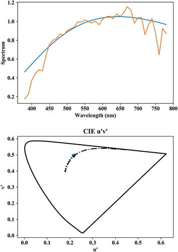
Fig. 2. Plot of spectral data in REF.

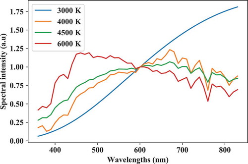
Fig. 3. Monte Carlo–generated individual XYZ color matching functions.

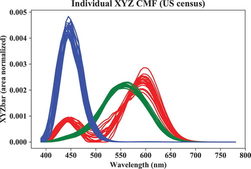
Fig. 4. Output of plot_color_data().

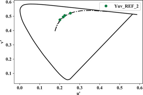
Fig. 5. Plot of u’v’ coordinates of CIE TCS8 before (red circles) and after (blue diamonds) a von Kries CAT from a 3000 K blackbody radiator to CIE illuminant D65.

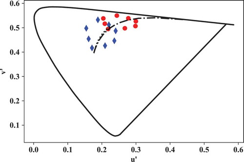
Fig. 6. Plot of CIE TCS8 samples in CIECAM02 J, a_M, b_M. Red circles: default viewing conditions, blue diamonds: user-defined conditions.

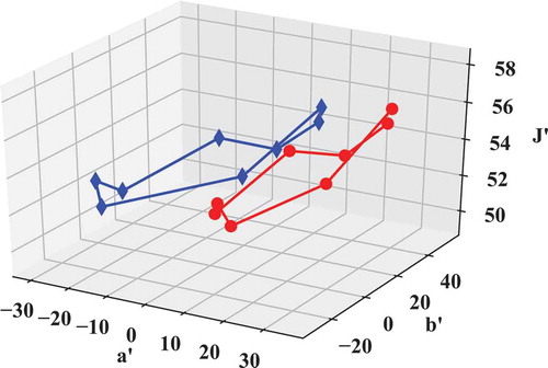
Fig. 7. TM30-like graphic output of the color rendition properties of CIE illuminant F4. Top left: SPD with inline text of CCT, Duv, R_f, R_g, and R_t (metameric uncertainty index). Mid row, left: R_fhi index values for hue bins 1–16. Mid row, right: same but base color shifts predicted by a vector field model. Bottom row left and right: local hue hue and chroma shifts. Top right: color graphic icon. Bottom right: base color shifts predicted by a vector field model together with the Munsell-5 hue lines.

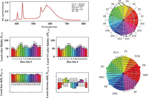
Fig. 8. TM30-like graphic output of the color rendition properties of CIE illuminant F4. Similar to Fig. 7 but with hue coloring turned off in the right graphs and with base color shift vectors overlayed with lines representing the distortion of concentric chroma circles due to the specific color rendition properties of the test light source. Hue shift information is represented by the width and coloring of the lines: wider, more reddish lines represent larger hue shifts.

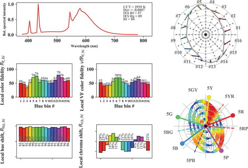
Fig. 9. Four monochromatic leds generated with spd_builder().

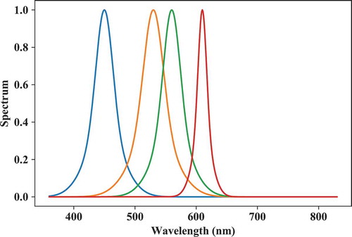
Fig. 10. Two phosphor-type and one monochromatic LED spectrum generated with spd_builder().

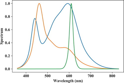
Fig. 11. Two phosphor-type LED spectra generated with spd_builder() for which the target chromaticity (CCT = 3500 K, Duv = 0) was inside the gamut spanned by its components.

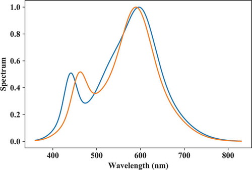
Fig. 12. Spectrum optimized from predefined, fixed component spectra for a CCT = 3500 K and IES TM30 R_f and R_g objective functions.

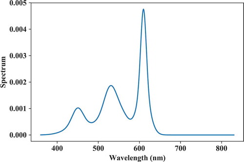
Fig. 13. Spectrum optimized from predefined, fixed component spectra for a CCT = 3500 K and IES TM30 R_f and R_g objective functions.

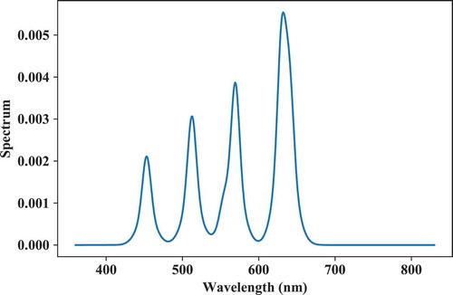
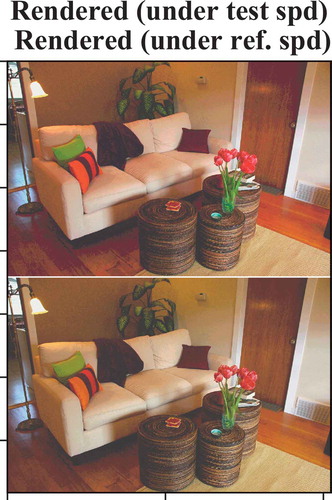
Fig. 14. Rendering results of simulated hyperspectral images. Top: using the 4000 K RGB LED test light source spectrum. Bottom: using the reference (D65) spectrum. A von Kries chromatic adaptation with degree of adaptation set to D = 1 has been applied.