The role of information sentiment in popularity on social media: a psychoinformatic and electroencephalogram study

Figures & data

Figure 1. The prime paradigm. A standard trial started with a fixation cross followed by a prime stimulus. Then, a blank screen was presented followed by targets.

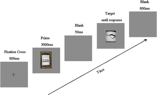
Figure 2. Behavioral results in Experiment 1. (a) Illustrated the mean ratings of valence and arousal for popular information/unpopular information. The ratings were assessed in a nine-likert scale. Error bars were 95% confidence interval. ‘***’ indicated p < 0.001. (b) Indicated the mean reaction time for three types of IAPS targets per prime. Abbreviation: HIAPS, IAPS targets with high sentiment; LIAPS, IAPS targets with low sentiment; NIAPS, neutral white stimuli. Error bars were 95% confidence interval. ‘*’ indicated p < 0.05. The unit for RT was milliseconds.

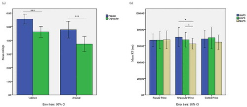
Figure 3. Electrode distributions. The scalp electrodes were illustrated. Red, yellow and green indicated frontal, central and parietal areas, respectively. Left and right mean left/right brain hemispheres.

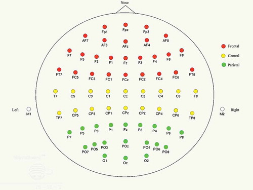
Figure 4. The priming effect of the target-locked ERP amplitudes at frontal, central and parietal areas within the time window 0–1000 ms. Abbreviations: HIAPS, IAPS targets with high sentiment; LIAPS, IAPS targets with low sentiment; NIAPS, neutral white stimuli. X and Y axes indicated the types of targets and 95% confidence interval of mean amplitudes, respectively. The unit of Y-axis was µV. Blue, green and yellow circles indicated the control, popular and unpopular primes, respectively. The symbol ‘*’ and ‘**’ means p < 0.05 and p < 0.01, respectively.

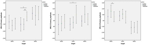
Figure 5. Grand mean target-locked ERP amplitudes across subjects. The graph was an illustration of grand mean target-locked ERP amplitudes within the time window −100–1000 ms across subjects. X-axis was the time window with the unit of milliseconds; Y axis was the grand mean amplitudes with the unit of µV. (a) Indicated the grand mean amplitudes at channel POZ when the target was IAPS with high arousal and high valence. (b) Indicated the grand mean amplitudes at channel FZ when the target was IAPS with low arousal and low valence. The blue, red and yellow lines indicated the control, unpopular and popular primes, respectively.

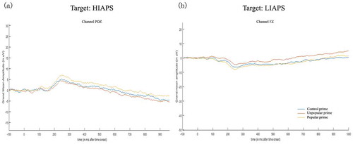
Figure 6. Topography of grand mean target-locked ERP amplitudes across subjects. It illustrated the scalp topography for target-locked ERP at 456 ms after the onset of target. The color bar was ranging from −20 to 20 µV. (a) Means when the target was IAPS with high sentiment, popular prime and unpopular prime evoked the target-locked ERP, mainly obviously different at parietal electrodes. (b) Means when the target was IAPS with low sentiment, popular/unpopular prime elicited the target-locked ERP, mainly different at frontal-central electrodes.

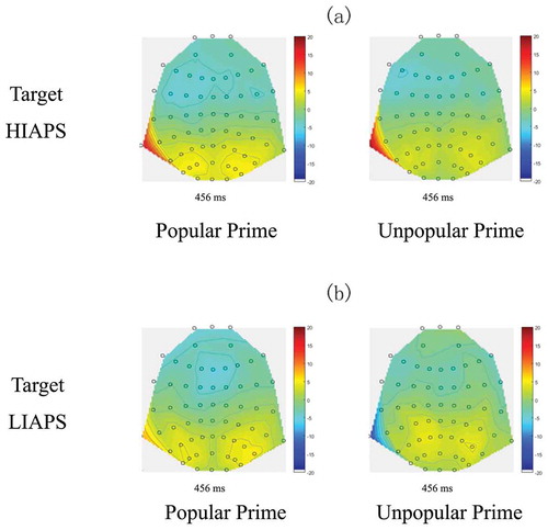
Table 1. Correlations between self-reported ratings and prime-locked ERP amplitudes.

	Frontal electrodes	Central electrodes	Parietal electrodes
Part I: Pearson correlations between valence and prime-locked ERP amplitudes
Positive	FP1 (r = 0.36*)	N/A	N/A
	FPZ (r = 0.35*)
	FP2 (r = 0.37*)
	AF3 (r = 0.34*)
	F7 (r = 0.31*)
Negative	FC3 (r = -0.35*)	N/A	N/A
Part II: Pearson correlations between arousal and prime-locked ERP amplitudes
Positive	FP2 (r = 0.36*)	CZ (r = 0.31*)	PZ (r = 0.32*)
	AF4 (r = 0.35*)	C6 (r = 0.46**)	P6 (r = 0.44**)
	F4 (r = 0.37*)		POZ (r = 0.32*)
	F6 (r = 0.53**)
	FCZ (r = 0.32*)
Negative	F5 (r = -0.39**)	T8 (r = -0.35*)	P7 (r = -0.34*)
	FT7 (r = -0.38*)	TP7 (r = -0.30*)	P5 (r = -0.30*)
	FC5 (r = -0.42**)	CP5 (r = -0.42**)	P8 (r = -0.31*)
	FT8 (r = -0.33*)	TP8 (r = -0.29*)	PO7 (r = -0.39**)
			PO5 (r = -0.39**)

Notes: the symbol ‘*’ and ‘**’ mean p < 0.05 and p < 0.01, respectively.

Figure 7. Scatter graphs for Pearson correlations between self-report ratings and prime-locked ERP amplitudes. (a) indicated the positive correlations between prime-locked amplitudes with valence ratings of popular/unpopular information at channels FP1, FPZ, FP2. (b) Indicated the positive correlations between prime-locked amplitudes and arousal ratings of popular/unpopular information at channels F6, C6, P6. (c) Indicated the negative correlations between prime-locked ERP amplitudes and arousal ratings of popular/unpopular information at channels F5, CP5, PO5. Linear regression models and tendency lines were shown for each correlation graph. The linear R² was shown on the top right of each correlation graph. The X-axis was the rating scores; Y-axis was mean prime-locked ERP amplitudes for the time window 0–1000 ms. The unit for amplitudes was µV.