Berry distributions on coffee trees cultivated under high densities modulate the chemical composition of respective coffee beans during one biannual cycle

Figures & data

Figure 1. Mean and standard error values of sum of berries per plant distributed over vertical (A and C) and horizontal profile, on the second-order axes (B and D), in the first production year (2010). The sum of berries collected in the first harvest is shown on upper line and sum of berries collected in the second and third harvests is represented at lower line. Plants were cultivated under two planting patterns (Q – square and R – rectangular) and densities (10,000 and 6000 plants ha⁻¹).

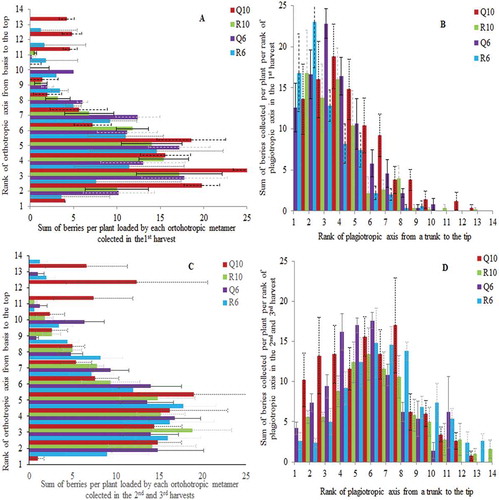
Table 1. ANOVA P-values for the effects of planting density (Dens, 10,000 and 6000 plants ha⁻¹), planting pattern (PP, Q – square and R – rectangular) and rank of orthotropic and plagiotropic axes on the berry distribution in the first production year during the first and later harvests (second + third).

	First		Second + Third
Harvest	Othotropic	Plagiotropic	Othotropic	Plagiotropic
Dens	0.0475	0.6757	0.423	0.703
PP	0.0303	0.2519	0.3577	0.0124
Dens × PP	0.7344	0.8229	0.1536	0.9297
Along axis	<0.0001	<0.0001	<0.0001	<0.0001
First versus second + third harvest			0.4975	0.0755

P-values < 0.05 were considered significant and marked in bold.

Figure 2. Mean and standard error values of sum of berries per plant distributed over vertical (A and C) and horizontal profile, on the second-order axes (B and D), in the second production year (2011). The sum of berries collected in the first harvest is shown on upper line and sum of berries collected in the second harvest is represented at lower line. Plants were cultivated under two planting patterns (Q – square and R – rectangular) and densities (10,000 and 6000 plants ha⁻¹).

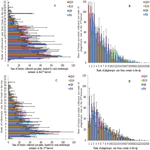
Table 2. ANOVA P-values for the effects of planting density (Dens, 10,000 and 6000 plants ha⁻¹), planting pattern (PP, Q – square and R – rectangular), occurrence over the 40-cm-thick layers and rank of orthotropic and plagiotropic axes on the berry distribution in the second production year during the first and second harvests.

	First		Second
Harvest	Othotropic	Plagiotropic	Othotropic	Plagiotropic
Dens	0.0019	0.001	0.0011	0.0007
PP	0.0009	<0.0001	0.0172	0.0005
Dens × PP	0.9665	0.9341	0.5232	0.429
Along axis	<0.0001	<0.0001	<0.0001	<0.0001
Layer	<0.0001	<0.0001	<0.0001	<0.0001
First versus second harvest			<0.0001	<0.0001

P-values < 0.05 were considered significant and marked in bold.

Table 3. Means (g 100 g⁻¹) and Tukey test following by ANOVA P-values for the effects of production year (PY, first and second after the low tree pruning), planting densities (Dens, 10,000 and 6000 plants ha⁻¹) and patterns (PP, Q – square and R – rectangular) on chemical compounds of coffee beans.

Factors		Variables
		PRO		LIP		TS		SAC		RS		CAF		PC		CGA
Means (g 100 g^−1)
PY	First	14.09	A	15.15	A	7.34	A	6.96	B	0.38	A	1.39	B	5.69	A	8.61	A
	Second	14.37	A	14.72	B	7.52	A	7.20	A	0.33	B	1.49	A	5.76	A	7.34	B
Dens	Q	14.34	A	15.05	A	7.49	A	7.13	A	0.36	A	1.46	A	5.78	A	8.03	A
	R	14.15	A	14.80	A	7.39	A	7.04	A	0.35	A	1.43	A	5.67	B	7.86	A
PP	10	14.50	A	14.96	A	7.49	A	7.18	A	0.34	A	1.48	A	5.70	A	7.87	A
	6	13.98	B	14.89	A	7.39	A	6.99	A	0.37	A	1.41	B	5.76	A	8.02	A
ANOVA
		P-values
PY		0.6480		0.0671		0.1023		0.0384		0.0016		0.0007		0.2425		<0.0001
Dens		0.0013		0.6407		0.1309		0.0754		0.1145		0.0003		0.2689		0.2100
PP		0.2191		0.3817		0.3714		0.4371		0.4977		0.4078		0.0448		0.0622
PY × Dens		0.1128		0.0660		0.3239		0.4071		0.2867		0.6257		0.6047		0.4099
PY × PP		0.3192		0.7416		0.2740		0.3718		0.1504		0.2049		0.5612		0.5726
Dens × PP		0.9973		0.5442		0.7443		0.6992		0.6554		0.1424		0.8272		0.6189
PY × Dens × PP		0.7096		0.6717		0.7233		0.7755		0.5775		0.9637		0.1997		0.6535

P-values < 0.05 were considered significant and marked in bold.

Table 4. Means (g 100 g⁻¹) and Tukey test following by ANOVA P-values for the effects of harvest periods, planting densities (Dens, 10,000 and 6000 plants ha⁻¹) and patterns (PP, Q – square and R – rectangular) on chemical compounds of coffee beans in the first production year.

Factors		Variables
		PRO		LIP		TS		SAC		RS		CAF		PC		CGA
Means (g 100 g^−1)
Harvest	First	14.63	A	14.34	B	7.40	A	7.03	A	0.37	A	1.41	A	5.71	A	8.61	AB
	Second	13.99	B	15.45	A	7.04	B	6.67	B	0.37	A	1.38	A	5.78	A	8.89	A
	Third	13.67	B	15.65	A	7.55	A	7.15	A	0.40	A	1.40	A	5.61	A	8.37	B
Dens	10	14.22	A	15.04	A	7.49	A	7.10	A	0.38	A	1.42	A	5.67	A	8.55	A
	6	13.99	A	15.24	A	7.23	B	6.84	B	0.38	A	1.37	B	5.71	A	8.67	A
PP	Q	14.08	A	15.27	A	7.46	A	7.05	A	0.41	A	1.39	A	5.77	A	8.79	A
	R	14.10	A	15.05	A	7.25	A	6.88	A	0.36	B	1.40	A	5.63	A	8.47	A
ANOVA
		P-values
Harvest		0.0012		<0.0001	0.0079			0.0105		0.1950		0.7555		0.3547		0.0773
Dens		0.3770		0.1621	0.0397			0.0337		0.8418		0.0433		0.6516		0.5071
PP		0.6543		0.1536	0.0677			0.1259		0.0041		0.6283		0.1458		0.0946
Harvest × Dens		0.9802		0.0655	0.6095			0.6231		0.0344		0.6192		0.3092		0.8697
Harvest × PP		0.9708		0.4090	0.5446			0.4184		0.4767		0.7029		0.3678		0.3410
Dens × PP		0.3998		0.7369	0.9144			0.9928		0.7293		0.1530		0.4795		0.5460
Harvest × Dens × PP		0.8721		0.6902	0.1555			0.1874		0.2960		0.9690		0.3878		0.3507

P-values < 0.05 were considered significant and marked in bold.

Table 5. Means (g 100 g⁻¹) and Tukey test following by ANOVA P-values for the effects of harvest periods, planting densities (Dens, 10,000 and 6000 plants ha⁻¹) and patterns (PP, Q – square and R – rectangular) on chemical compounds of coffee beans in the second production year.

Factors		Variables
		PRO		LIP		TS		SAC		RS		CAF		PC		CGA
Means (g 100 g^−1)
Harvest	First	14.36	A	15.64	A	6.99	B	6.68	B	0.31	A	1.40	B	5.76	A	7.24	A
	Second	14.38	A	14.29	B	7.77	A	7.44	A	0.33	A	1.53	A	5.76	A	7.39	A
Dens	10	14.70	A	14.90	A	7.54	A	7.23	A	0.31	A	1.52	A	5.72	A	7.38	A
	6	13.96	B	14.50	B	7.51	A	7.16	A	0.35	A	1.45	B	5.81	A	7.30	A
PP	Q	14.54	A	14.88	A	7.52	A	7.20	A	0.32	A	1.51	A	5.79	A	7.44	A
	R	14.20	A	14.55	B	7.53	A	7.20	A	0.33	A	1.47	A	5.72	A	7.25	A
ANOVA
		P-values
Harvest		0.2342		<0.0001		<0.0001		<0.0001		0.5066		<0.0001		0.8319		0.2970
Dens		<0.0001		0.0026		0.8371		0.6491		0.1545		0.0008		0.1085		0.5593
PP		0.1694		0.0092		0.9694		0.9827		0.8256		0.1444		0.0847		0.1049
Harvest × Dens		0.3933		0.0370		0.4628		0.6271		0.1952		0.5736		0.7573		0.5652
Harvest × PP		0.5218		0.9106		0.7448		0.7967		0.6940		0.2863		0.1535		0.0585
Dens × PP		0.3996		0.7164		0.4015		0.4036		0.8215		0.2957		0.1207		0.8170
Harvest × Dens × PP		0.1403		0.8564		0.3832		0.4300		0.7891		0.4360		0.8729		0.1646

P-values < 0.05 were considered significant and marked in bold.

Table 6. Means (g 100 g⁻¹) and Tukey test following by ANOVA P-values for the effects of vertical profile localization of coffee berries over the 40-cm-thick layers, planting densities (Dens), and patterns (PP) on chemical compounds of coffee beans in the second PY.

Factors		Variables
		PRO		LIP		TS		SAC		RS		CAF		PC		CGA
Means (g 100 g^−1)
Layer	1	14.88	A	14.60	A	7.60	A	7.30	A	0.30	A	1.54	A	5.69	B	7.25	A
	2	13.92	B	14.82	A	7.45	A	7.11	A	0.34	A	1.45	B	5.81	A	7.43	A
Dens	10	14.70	A	14.90	A	7.54	A	7.23	A	0.31	A	1.52	A	5.72	A	7.38	A
	6	13.96	B	14.50	A	7.51	A	7.16	A	0.35	A	1.45	B	5.81	A	7.30	A
PP	Q	14.54	A	14.88	A	7.52	A	7.20	A	0.32	A	1.51	A	5.79	A	7.44	A
	R	14.20	B	14.55	A	7.53	A	7.20	A	0.33	A	1.47	A	5.72	A	7.25	A
ANOVA
		P-values
Layer		<0.0001		0.2703		0.2860		0.1573		0.1072		0.0015		0.0133		0.0771
Dens		<0.0001		0.1017		0.5930		0.4177		0.1677		0.0010		0.1069		0.4290
PP		0.0239		0.1991		0.6972		0.7151		0.7848		0.1259		0.1528		0.1191
Dens × PP		0.3832		0.5404		0.3218		0.3093		0.9602		0.4418		0.1242		0.7202
Dens × Layer		0.1861		0.8433		0.0433		0.0275		0.4233		0.3296		0.2020		0.6425
PP × Layer		0.0344		0.9001		0.7395		0.6790		0.5985		0.3925		0.8811		0.0330
Dens × PP × Layer		0.8612		0.2024		0.0943		0.1034		0.5294		0.4014		0.8299		0.4557

P-values < 0.05 were considered significant and marked in bold.