An integrated mixed integer linear programming model for resilient and sustainable natural gas supply chain

Figures & data

Figure 1. Simple layout of a natural gas supply chain.

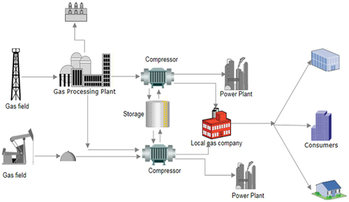
Figure 2. Case study system layout with additional workflow (adopted from (Emenike and Falcone 2020)).

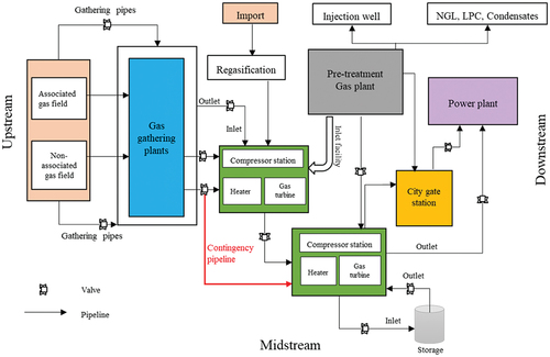
Table 1. Optimization scenarios.

Scenario	Description	Condition
Steady state
0	Baseline scenario	No relief pipeline
1	Shutdown with redundancy	Relief pipeline operating with no pressure variation
2	Flow constraint in extended time	Flow constraint introduced when redundancy is operating
3	No flow constraint in extended time	No corresponding upper & lower bound limits
Transient state
4	Pressure surge from plant closure	Trapped gas undergoes pressure variation
5	Prolonged inlet & outlet nodes closure	Unexpected pressure build-up

Table 2. Case study: Reference parameters.

Symbol	Description	Value	Unit
$t$	Duration of each time interval	1	days
$T$	Total number of times in the planning horizon	30	days
$d\mathrm{\_}{a}_{\left(m,t\right)}$	Demand for gas for power plant consumers $m$	360	mmscfd
$\theta P_{\left(p\right)}^{max}$	Maximum proportional capacity expansion rate	1.5
$\theta P_{\left(p\right)}^{min}$	Minimum proportional capacity expansion rate	1.3
$In{c}_{\left(p,t\right)}$	Capacity of plant $p$ before expansion	400	mmscfd
${\delta }_{\left(k\right)}$	Minimum offline time	2	days
${\mathrm{O}}_{\left(k\right)}$	Maximum offline time after the shutdown of plant $k$	52	days
${\mathrm{\Psi }}_{\left(k\right)}$	Minimum online time after the startup of plant $k$	4	days
$S_{\left(k\right)}^{max}/S_{\left(k\right)}^{min}$	Max/Min flow rates	300/200	mmscfd

Figure 3. Baseline flow rate during the planning horizon (in days).

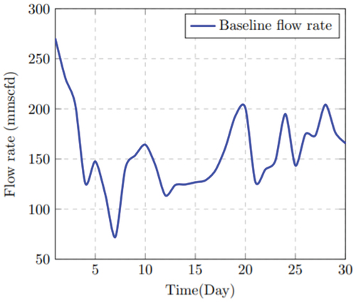
Figure 4. Performance level of compressor k with respect to the mass flow rate under the baseline scenario (Scenario 0).

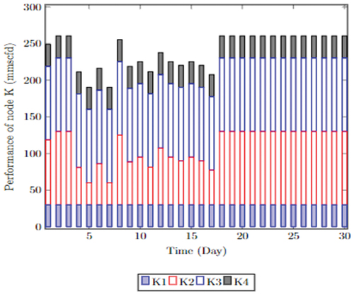
Figure 5. Flow rate with no pressure drop at fixed mass flow rate.

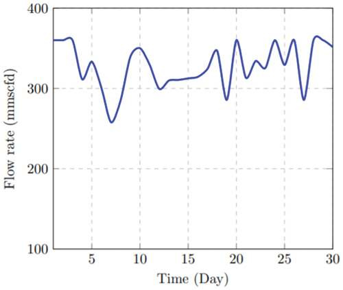
Figure 6. Flow rate with no pressure drop at varying mass flow rates.

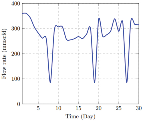
Figure 7. Performance level of the compressor mass flow rate when the plant starts operating after a shutdown (Scenario 1).

Figure 8. Steady state with flow constraint (Scenario 2).

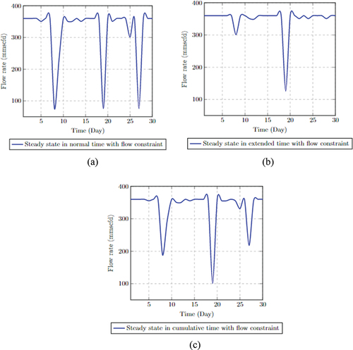
Figure 9. Flow rate without flow constraint in extended time (Scenario 3).

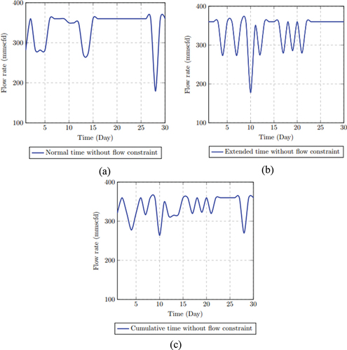
Figure 10. Pressure variation when mass flow rate is maximum.

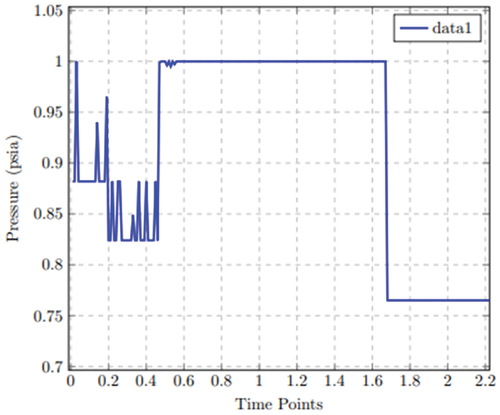
Figure 11. Pressure variation when mass flow rate is minimum.

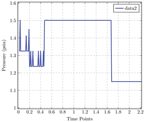
Figure 12. Outlet pressure interaction when compressibility factor equals 1.

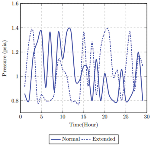
Figure 13. Outlet pressure when compressibility factor is lower than 1.

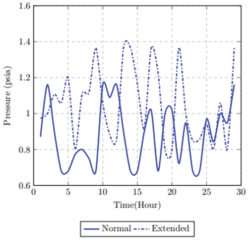
Table 3. Pressure activity in Mainline during disruption.

Description	Performance	Pressure (psi)	Behavior
Mainline pipe node when the valve is closed at inlet node.	Increased at 11:54	1389	Stable
	Decreased at 17:48	1316	Stable
	Decreased at 23:42	1276	Stable
Opening of the relief valve and re-opening of mainline valve.	Decreased at 11:54	1260	Stable
	Increased at 17:48	1330	Stable
	Increased at 23:42	1375	Stable

Figure 14. Pressure bound limit in extended time.

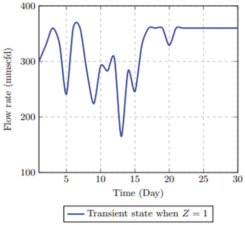
Figure 15. Pressure bound limits, higher compressibility factor in extended time.

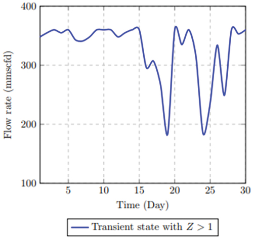
Table 4. Comparison of throughput across different cases.

State	Description	Throughput (mmscfd)
Steady	Optimized flow obtained if the capacity of node k is the same for all period in the planning horizon.	327.67
	Optimized flow is obtained if the capacity of node k varies at different rates in the planning horizon.	276.38
	Optimized flow is obtained when the flow constraint is introduced.	336.078
	Optimized flow is obtained when the flow constraint is removed.	336.90
Transient	Pressure variation in extended time.	200.38
	When compression factor equals 1 with an extended time.	321.17
	When pressure bound limit is introduced in extended time.	323.37
	The compression factor is increased in extended time.	327.03

Emenike, S.N., and G. Falcone. 2020. A Review on Energy Supply Chain Resilience through Optimization. Renewable and Suatainable Energy Reviews 134: 110088. doi:10.1016/j.rser.2020.110088.

 Web of Science ®Google Scholar