Optimal design and techno-economic analysis of hybrid renewable energy systems: A case study of Thala city, Tunisia

Figures & data

Table 1. Previous research, system architecture, and key findings summary.

Reference	Hybrid architecture	Mode	Location	Application	Findings
(Mulenga et al. 2023)	PV/diesel	Off-grid	Chilubi Island, Zambia	Rural electrification	- PV/diesel/battery, COE of 0.18 US$/kWh
(Amole et al. 2023)	Grid only, PV only, and PV-grid	On-grid	Oyo State, Nigeria	Remote village electrification	- PV grid system is the best system with an LCOE of 0.19 US$/kWh
(Krishnamoorthy et al. 2020)	PV/biomass with different batteries for storage (lead acid, Li-ion, flow battery)	Off-grid	Korkodu, India	Village electrification	- Li-ion is the cost-effective storage technology with 0.22 US$/kWh COE and 190,507 US$/kWh NPC
(Agyekum et al. 2022)	Hydrogen/Batteries	Off-grid	Upper East region of Ghana	agricultural activities electrification	- Hydrogen/Batteries is the winning system with 0.06 US$/kWh LCOE and 18,180 US$ operation costs.

The rest of this paper is structured into the following sections: Section 2 presents the methodology, providing details about HOMER models and their inputs, such as the load profile, the system components and configurations, and the mathematical modeling of the proposed HES. Section 3, describes and discusses the techno-economic and environmental results. Finally, the conclusions are summarized in section 4.

Figure 1. Methodology of the research work.

Figure 2. Simplified flowchart of HOMER pro optimization algorithm.

Figure 3. Single-line diagram of the renewable energy system.

Figure 4. Geographic location of Thala.

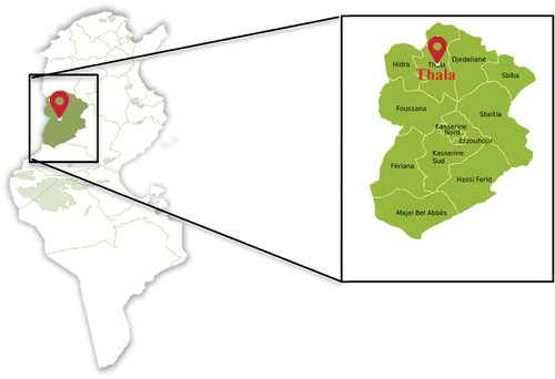
Table 2. Case study characteristics.

Municipality	Thala
Governorate	Kasserine
Country	Tunisia
Latitude	35°34’20.78“N
Longitude	8°40’13.12“E
Total population	39,400
Population density	51.4/km^2

Table 3. Monthly climate data of Thala.

	Wind power density (W/m²)	Av wind speed (m/s)	Solar energy (kWh)	Av sun hours	Rainy days	Rainfall (mm)	Max T (°C)	Min T (°C)	Av T (°C)
Jan	400	6.2	3	10	4.1	35.5	19	3	11
Feb	470	6.5	3.9	10.9	3.6	27.9	21	6	13.5
Mar	490	6.2	5.2	121	4.9	35.5	27	7	17
Apr	470	6.1	6.4	3.11	5	30.5	30	8	19
May	380	5.7	7.2	4.11	5.3	30.5	42	12	27
Jun	320	4.9	7.7	4.51	3.5	20.3	51	26	38.5
Jul	300	4.9	7.9	4.31	1.9	10.2	56	31	43.5
Aug	280	4.75	7.1	3.41	4.1	17.8	59	33	46
Sep	290	5.1	5.6	2.41	6.4	33.0	51	28	39.5
Oct	320v	5.7	4.3	1.31	5.1	33.0	32	15	23.5
Nov	325	6.1	3.2	0.39	3.7	28	27	10	18.5
Dec	400	6.5	2.7	9.8	3.7	30.5	19	6	12.5

Figure 5. Hourly power demand pattern on two days of maximum power consumption during 2019 and 2020 in Thala city (A.R.C. 2009).

Table 4. Average demand of Thala city (Llc 2022).

Year	2010	2011	2012	2013	2014	2015	2016	2017	2018	2019	2020
Consumption (MW)	0.99	1.13	1.28	1.43	1.59	1.82	2.00	2.19	2.37	2.60	3.88

Table 5. The power rating of different appliances in Thala city (Power Consumption Table 2003).

Appliance	Power (W)	Number	Average (hours/day)	Average (Wh/day)
Light	15	20	7	2100
TV	100	1	6	600
Radio	1	1	3	3
Laptop/computer	70	1	5	350
Phone charger	5	3	6	90
Washing machine	600	1	2	1200
Water heater	1500	1	4	6000
Fridge/freezer	150	1	24	3600
Total Wh/day				13943

Figure 6. Annual mean wind speed (Elamouri et al. 2008).

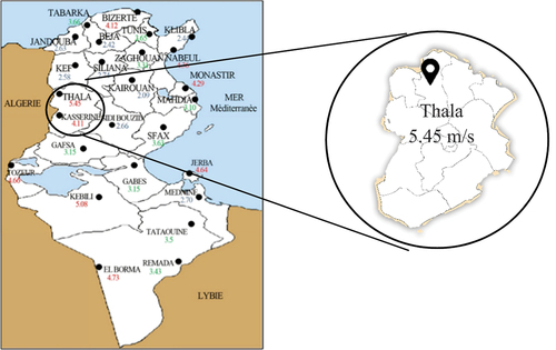
Figure 7. Hourly wind speed in Thala city over 30 years (1990‒2020).

Figure 8. Monthly average wind speed variation with elevation.

Figure 9. Modern three-phase extraction process of olive oil.

Table 6. Properties of olive mill by-products (Al-Najjar et al. 2022).

	Moisture	Ash	Total solids (TS)/FM	Volatile solids (VS)/DM	Oil	Protein	Phenols
Olive leaves	50%	2.5%	50%	-	3%	7%	2.4%
OMWW	92.9%	1.5%	78.6 mg/l	44 g/L	0.3%	8.3 g/L	1‒11%
OP	48‒54%	8.8%	900 g/L	68.2%	0.08%	5‒6%	0.1‒4%

FM: Fresh matter, DM: Dry matter

Table 7. Biomass availability and biogas yield production in Thala city (Milanese et al. 2014; Shakeri et al. 2017).

Biomass resources	OMWW	OP	Olive leaves
Availability (ton)^1	7.8	3.3	0.36
Total (ton/day)^1	65	27.5	3
Biogas yield (m^3/kg)/FM	0.06	0.082	0.118
Total biogas (m^3/day)^1	3900	2255	354
Energy yield (MWh/day)	39	22.5	3.5

FM: Fresh material, ¹ per season

Figure 10. Simplified lead-acid battery charging profile.

Figure 11. Carbon footprint from different processes within the olive oil production cycle (Feliciano, Maia, and Gonçalves 2014).

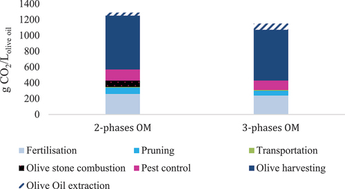
Table 8. Technical properties of the selected components.

Wind turbine EOX M-21	Max. hub height	32 m
	Rated power	100 kW
	Lifetime	25
	Rated wind speed	10 m/s
	Initial cost	100,000 US$/kW
	Replacement cost	80,000 US$/kW
	O&M cost	400 US$/kW
Biomass gasifier	Lifetime (hours) Rated capacity	15,000 3,056 (kg/day)
	Initial cost	40,000 US$
	Replacement cost	12,000 US$
	O&M cost	2 US$/op.hour
OPzV lead acid battery	Nominal voltage	2 V
	Nominal capacity	0.7 kWh
	Initial cost	1000 US$
	Replacement	1000 US$
	O&M	200 US$/year
Pumped hydro storage	Nominal voltage	240 V
	Maximum electrical charge	2500 Amp hours
	Initial cost	200 US$/kWh
	O&M	50 US$/kWh
	Lifetime	80 years

Figure 12. The power curve of the selected wind turbine (eocycle 2023).

Figure 13. Pumped storage hydropower technology.

Table 9. Simulation scenarios.

Scenarios	Assumptions
Grid-connected including Batteries (ON-Grid_BATT) or PHS (ON-Grid_PHS).	A hybrid power plant that combines olive mill wastes and wind energy sources connected to the main power grid and incorporates a Pumped Hydro Storage system/Batteries This scenario optimizes the utilization of renewable energy, reduces the reliance on fossil fuel-based backup generation, and contributes to a more sustainable and resilient grid system.
Grid-connected without storage devices (ON-Grid_Only)	Hybrid power plant with olive mill wastes and wind energy sources directly connected to the main power grid. It relies on the immediate power supply to the grid, providing stability during active renewable energy periods but requiring fossil fuel backup during low renewable energy periods.
Standalone system including Batteries (OFF-Grid_BATT) or PHS (OFF-Grid_PHS)	Hybrid power plant based on biomass and wind energy that operates independently of the main power grid. It includes batteries/PHS storage to store excess energy generated during periods of high production and utilize it during low or no generation periods. This configuration ensures a consistent and reliable power supply in remote areas with limited access to electricity, reducing the risk of power shortages and enhancing overall system efficiency.

Table 10. Optimization results - architecture, costs, and environmental impacts.

Optimization results
Scenario	Configuration		Architecture					Cost			Renewable fraction (%)	Emission CO2 (ton/year)
			WT (kW)	BG (kW)	Conv (kW)	BATT (Unit)	PHS (kW)	NPC (k US$)	LCOE (US$)	OC (kUS$/year)
Reference		Grid only	N/A	N/A	N/A	N/A	N/A	2130	0.063	164	0	1427
ON-Grid_BATT	Conf_1	Wind/Batt/Grid/Converter	3*100	N/A	5.08	35	N/A	530.10	0.053	26.26	73.0	380.3
	Conf_2	BG/Batt/Grid/Converter	N/A	100	7.81	100	N/A	548.20	0.056	31.39	25.6	1000.8
ON-Grid_PHS	Conf_3	Wind/BG/PHS/Grid/Converter	2*100	100	5.08	N/A	245	501.54	0.042	21.50	76.2	342.5
	Conf_4	BG/PHS/Grid/Converter	N/A	100	25	N/A	245	671.62	0.065	2.5	2.5	1390
ON-Grid_Only	Conf_5	Wind/BG/Grid	3*100	100	N/A	N/A	N/A	298.68	0.035	13.82	57.9	614.6
	Conf_6	Wind/Grid	5*100	N/A	N/A	N/A	N/A	564.52	0.061	25.13	80.9	271.1
OFF-Grid_BATT	Conf_7	Wind/BG/Batt/Conv	3*100	100	3.13	40	N/A	596.00	0.068	39.84	100	200
	Conf_8	BG/Batt/Conv	N/A	100	5.08	35	N/A	821.62	0.072	45.26	100	124
OFF-Grid_PHS	Conf_9	Wind/BG/PHS/Conv	2*100	100	5.08	N/A	254	738.54	0.070	39.83	100	118
	Conf_10	BG/PHS/Conv	N/A	100	6.25	N/A	735	3760.1	0.120	195.6	100	207

Figure 14. Cost-optimal configurations design for the On-grid_BATT scenario: left (Wind/Batteries/Grid/Converter); right (Wind/BG/Batteries/Grid/converter).

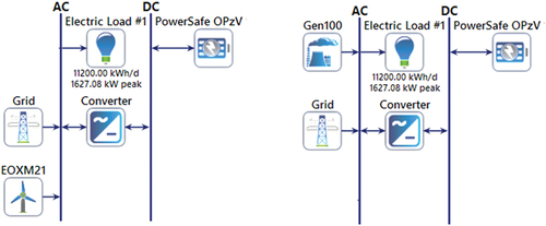
Figure 15. Monthly average electric production: (A) Wind/Batteries/Grid/converter, (B) Biomass/Batteries/Grid/converter.

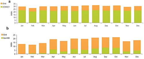
Figure 16. (A) energy purchased from the grid and (B) energy sold to the grid for the first configuration of Wind/Batteries/grid/Converter.

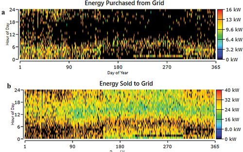
Figure 17. (A) energy purchased from the grid and (B) energy sold to the grid for the second scenario BG/Batteries/grid/Converter.

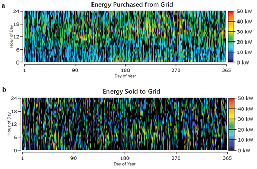
Figure 18. Cost-optimal configurations design for the On-grid_PHS scenario left (Wind/BG/PHS/Grid/Converter); right (Bg/phs/grid/converter).

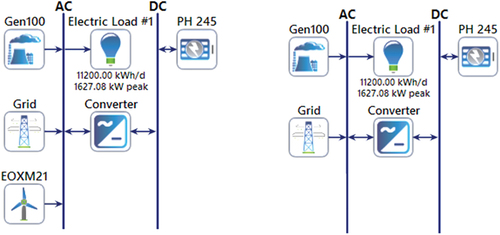
Figure 19. Monthly average electric production: (A) Wind/Biomass/PHS/Grid/converter (B) Biomass/PHS/Grid/converter.

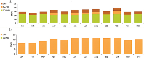
Figure 20. Renewable energy integration: Wind/BG/PHS/Grid/Converter.

Figure 21. Cost-optimal configurations designed for the On-grid without storage scenario, left (Wind/BG/Grid/Converter); right (Wind/Grid/converter).

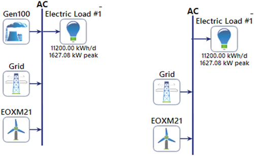
Figure 22. Monthly average electric production: (A) Wind/BG/Grid, (B) Wind/Grid.

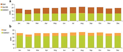
Figure 23. Electricity sold to the grid.

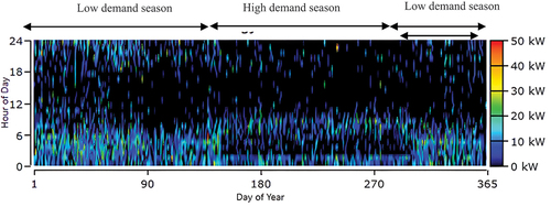
Figure 24. Cost-optimal configurations design for the off-grid _BATT scenario, left (Wind/BG/Batteries/Converter); right (Bg/batteries/converter).

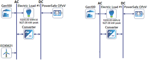
Figure 25. Monthly average electric production of Wind/BG/Batteries/converter.

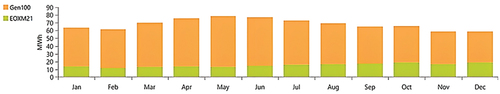
Figure 26. Hourly electric production, (A) generic 100 kW biogas gasifier, (B) EOX M-21 kW wind turbine.

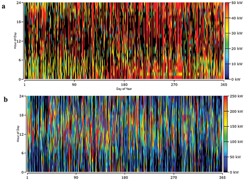
Figure 27. Cost-optimal configurations design for the off-grid _PHS scenario, left (Wind/BG/PHS/Converter); right (Bg/phs/converter).

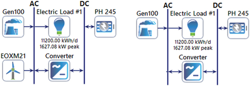
Figure 28. Monthly average electric production of Wind/BG/PHS/Converter configuration.

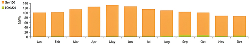
Figure 29. NPC (left) and LCOE (right) comparison of all the studied systems.

Table 11. Economic comparison with the base system.

Configuration	ROI	IRR	Simple Payback (Years)
Conf_1	72%	12.5%	7.3
Conf_2	68%	14%	8
Conf_3	88%	15%	7.8
Conf_4	43%	7%	12
Conf_5	110%	17%	7.2
Conf_6	63%	12%	8.6
Conf_7	58%	13.5%	13
Conf_8	42%	5%	13
Conf_9	45%	8%	15
Conf_10	−6%	14%	18

Table 12. Sensitivity analysis variables.

Sensitivity variables	Values
Nominal discount rate (NDR%)	8, 9, 10%
Biomass availability (ton/day)	35, 70
Annual scaled load demand (MWh/day)	11, 12, 13

Table 13. Impacts of NDR and project lifetime on the optimal configuration.

Architecture	Project lifetime (year)	NDR (%)	NPC (US$)	LCOE (US$)
Wind/BG/PHS/Grid/Converter	25	8	501,540	0.042
	25	9	514,078	0.046
	25	10	526,929	0.057

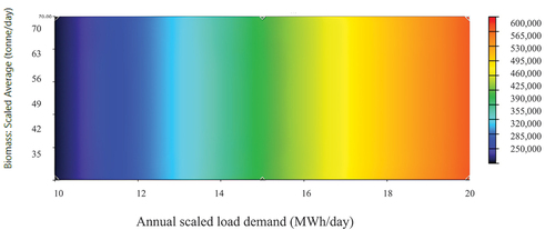
Figure 30. Sensitivity analysis: electric load average vs. biomass availability, NDR= 8%, project lifetime=25 years, surface plot: NPC, superimposed: LCOE.

Mulenga, E., A. Kabanshi, H. Mupeta, M. Ndiaye, E. Nyirenda, and K. Mulenga. 2023. Techno-economic analysis of off-grid PV-Diesel power generation system for rural electrification: A case study of Chilubi district in Zambia. Renewable Energy 203:601–11. doi:10.1016/j.renene.2022.12.112.

 Web of Science ®Google Scholar

Amole, A. O., S. Oladipo, O. E. Olabode, K. A. Makinde, and P. Gbadega. 2023. Analysis of grid/solar photovoltaic power generation for improved village energy supply: A case of ikose in Oyo State Nigeria. Renewable Energy Focus 44:186–211. doi:10.1016/j.ref.2023.01.002.

 Google Scholar

Krishnamoorthy, M., A. D. V. R. Periyanayagam, C. Santhan Kumar, B. Praveen Kumar, S. Srinivasan, and P. Kathiravan. 2020. Optimal sizing, selection, and techno-economic analysis of battery storage for PV/BG-based hybrid rural electrification system. IETE Journal of Research 68 (6):4061–76. doi:10.1080/03772063.2020.1787239.

 Web of Science ®Google Scholar

Agyekum, E. B., J. D. Ampah, S. Afrane, T. S. Adebayo, and E. Agbozo. 2022. A 3E, hydrogen production, irrigation, and employment potential assessment of a hybrid energy system for tropical weather conditions – combination of HOMER software, Shannon entropy, and TOPSIS. International Journal of Hydrogen Energy 47 (73):31073–97. doi:10.1016/j.ijhydene.2022.07.049.

 Web of Science ®Google Scholar

A.R.C, bureau d’étude. 2009. Final report of the engineering office A.R.C: Atlas du gouvernorat de Kasserine. 89. Ministere du transport et de l’equipement direction generale de l’amenagement du territoire. http://www.mehat.gov.tn/fileadmin/user_upload/Amenagement_Territoire/AtlasKasserineFrv2.pdf.

 Google Scholar

Llc, K. A. 2022. Data Collection Survey On Power Sector In Tunisia Final Report. Republic Tunisia Ministry of Industry, Energy and Mines Société Tunisenne de I ’ Electricite et du Gaz.

 Google Scholar

Power Consumption table. 2003. Retrieved September 20, 2023.

 Google Scholar

Elamouri, M., and F. B. Amar. 2008. Wind energy potential in Tunisia wind energy potential in Tunisia. Renewable Energy 33:758–768. doi:10.1016/j.renene.2007.04.005.

 Web of Science ®Google Scholar

Al-Najjar, H., H. El‐Khozondar, C. Pfeifer, and R. Al Afif. 2022. Hybrid grid-tie electrification analysis of bio-shared renewable energy systems for domestic application, sustainable cities and society. Sustainable Cities and Society 77:103538. doi:10.1016/j.scs.2021.103538.

 Web of Science ®Google Scholar

Milanese, M., A. De Risi, A. De Riccardis, and D. Laforgia. 2014. Numerical study of anaerobic digestion system for olive pomace and mill wastewater. Energy Procedia 45:141–49. doi:10.1016/j.egypro.2014.01.016.

 Google Scholar

Shakeri, P., Z. Durmic, J. Vadhanabhuti, and P. E. Vercoe. 2017. Products derived from olive leaves and fruits can alter in vitro ruminal fermentation and methane production. Journal of the Science of Food and Agriculture 97 (4):1367–72. doi:10.1002/jsfa.7876.

 PubMed Web of Science ®Google Scholar

Feliciano, M., F. Maia, and A. Gonçalves. 2014. An analysis of eco co-efficiency and GHG emission of olive oil production in northeast of Portugal. Int. J. Environ. Ecol. Eng. 8:347–52.

 Google Scholar

The wind power eocycle. the EOX M-21 data sheet. Retrieved July 15, 2023.

 Google Scholar