Assessment of Wooden Beams from Historical Buildings Using Ultrasonic Transmission Tomography

Figures & data

Figure 1. Scheme of passing: (a) i path through j element, (b) several paths through the object.

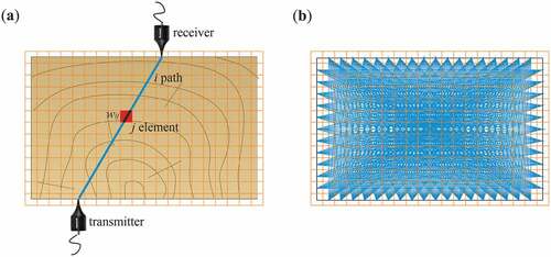
Figure 2. Location of the monastery of congregation of the sisters of St. Catherine located in Orneta: (a) city plan from 1627 from the collection of “Kriegsarchiv” in Stockholm, (b) urban layout according to Giesego early 19th century, (c) city plan from 1940, (d) panorama of the city in the 1930s (Hliwiadczyn, Cholewska, and Grunwald 2018).

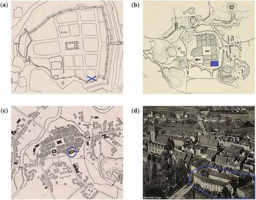
Figure 3. A rafter at the top of the roof of the monastery’s west wing. (Hliwiadczyn, Cholewska, and Grunwald 2018).

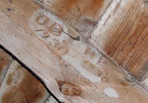
Figure 4. Photographs of the roof framework from the monastery of congregation of the sisters of St. Catherine in Orneta (Poland) before starting construction work (a-c) and when the works are carried out (d).

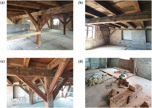
Figure 5. Laboratory models of wooden beams: (a) view of the beams, (b) dimensions of the beam, (c) cross-section of the tested beams #1–#3.

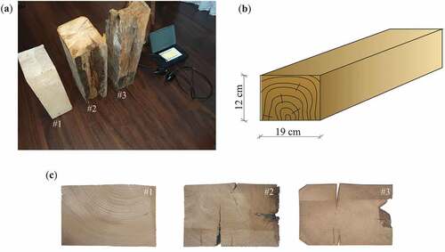
Figure 6. Experimental setup: (a) testing in through-transmission mode; (b) scheme of image reconstruction by ultrasonic tomography.

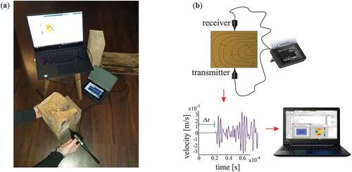
Figure 7. Configuration of the wave paths from transmitters (t) to receivers (r).

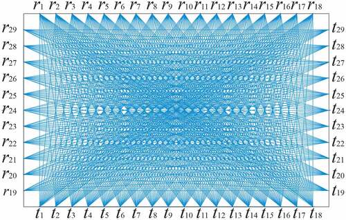
Table 1. Wave propagation velocities for beams #1-#3.

Wooden beam	vmin [m/s]	vmax [m/s]	Δv= vmax-vmin [m/s]	vavg [m/s]	SD [m/s]	CV [%]
#1	929.7	1637.0	707.3	1231.5	154.2	12.5
#2	632.7	1442.3	809.6	1093.3	137.0	12.5
#3	478.6	1842.5	1363.9	1462.3	293.4	20.1

Figure 8. Results obtained for beam #1: (a) top view of the beam, (a) ultrasonic tomography image, (c) side view of the beam.

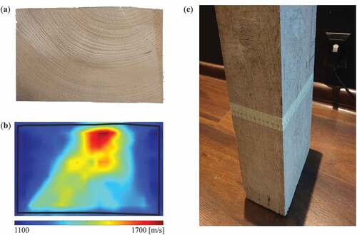
Figure 9. Results obtained for beam #2: (a) top view of the beam, (a) ultrasonic tomography image, (c) side view of the beam.

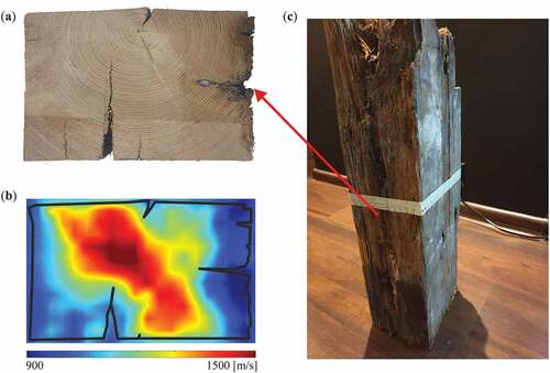
Figure 10. Results obtained for beam #3: (a) top view of the beam, (a) ultrasonic tomography image, (c) side view of the beam.

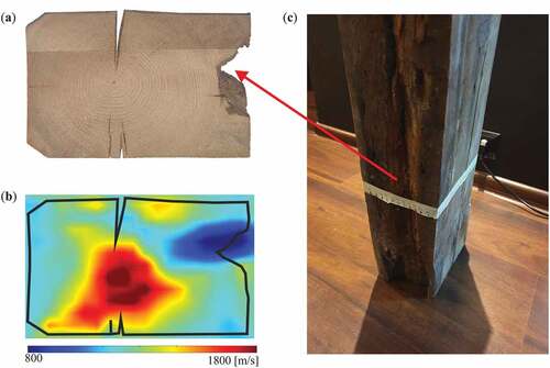
Figure 11. Rays of performed measurements with the 5% fastest waves marked in red.

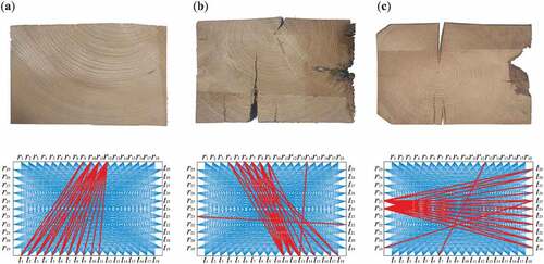
Table 2. Comparison of the velocity of waves propagating from two perpendicular walls.

Wooden beam		vavg [m/s]	vavg(1)/vavg(2) [-]
#1	wall 1	1286.9	1.19
	wall 2	1083.7
#2	wall 1	1117.4	1.09
	wall 2	1028.8
#3	wall 1	1455.3	1.02
	wall 2	1480.2

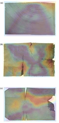
Figure 12. Determining the location of the pith form beams #1-#3.

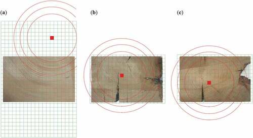
Figure 13. Ultrasound tomography maps: cross-sections (first row), idealized models, taking into account the location of the pith (second row), initial tomographic maps from Figures 8–10 (third row), the difference between the idealized maps and the initial maps (fourth row).

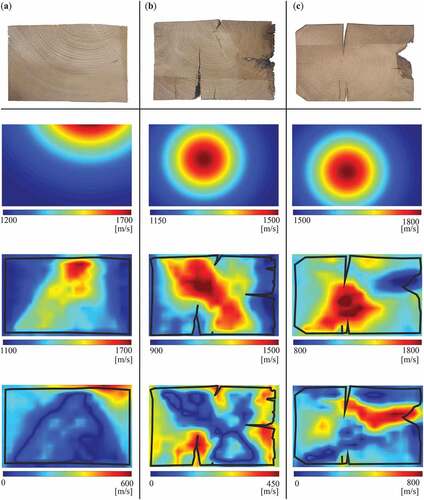
Figure 14. Final ultrasonic tomography maps imposed on cross-sections of tested beams.

Hliwiadczyn, S., M. Cholewska, and M. Grunwald. 2018. . Documentation of conservatoryResearch conservatory expertise and conservation work program, Vol II. concerning the interiors of the convent of the congregation of the sisters of St. Catherine in Orneta. Vol II. (Morąg) .

 Google Scholar