Building bridges: mycelium–mediated plant–plant electrophysiological communication

Figures & data

Figure 1. Petri dish design. Figure 1a illustrates the Petri dish cut in half with the agar on each side cut into the design to guide the mycelium across the agar gap in the center of the dish. Figure 1b depicts the Petri dish reassembled with spacers and rubber bands in place. Figure 1c represents the second method for reassembling the Petri dish using duct tape. Figure 1c also illustrates how the MycoGrow inoculant appeared on the agar after application.

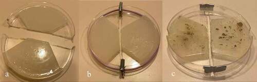
Figure 2. Mycelial bridging across the two islands of agar.

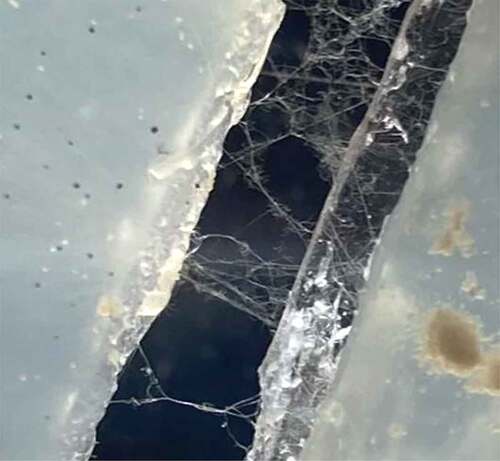
Figure 3. Setup testing platform This figure illustrates the testing platform used to aid in the isolation of the signal. The gap in the center of the platform kept the Petri dish off the surface of the table. This ensured the dish did not touch the testing table and further suspended the mycelial bridge in midair.

Figure 4. The mycelial bridge setups with direct inoculation of pea seeds and developed pea roots. Figure 4a depicts the pea seeds just after being coated with the Endo/Ecto MycoGrow Inoculant. Figure 4b depicts the same pea seeds, now covered with a damp paper towel to maintain moisture, the dish is now fastened together with tape at the ends while maintaining the necessary gap. The dish has also been fastened to the testing platform for stabilization. Figure 4c depicts direct inoculation of the pea’s root systems. Figure 4d depicts these same pea plants with the roots now covered by a damp paper towel to maintain moisture. This setup would also have been fastened to a testing platform, as seen in 4B.

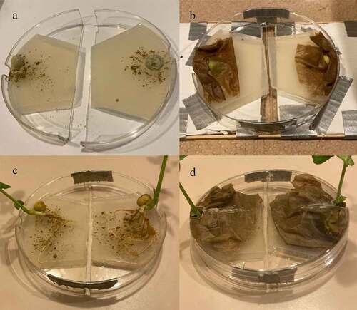
Figure 5. Examples of mycelial bridges when viewed under a microscope. This figure depicts the presence of mycelial bridges that the authors would visually confirm under the microscope prior to testing the setup.

Figure 6. Pea growing process.This figure depicts the process of growing pea plants from sprouting to testing. Figure 6a depicts the pea plants just beginning to sprout in a moist paper towel enclosure. Figure 6b depicts the same pea plants further along in the growth cycle with the above-mentioned angled setup. At this stage the pea plants are ready for testing. Figure 6c depicts the pea plant removed from the moist paper towel with the roots placed on one of the agar islands.

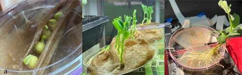
Figure 7. Experimental setup.We denote the side of the dish with the glass electrode and ground wire (6 and 7) as “Side A.” The plant and agar island on the side of the setup not being recorded is denoted “Side B.” The demarcation between side A and B is denoted with the dashed line – representing the gap between the two islands of agar. Each plant is fixed in position with tape and a beaker for stem support. Wax is used to secure the dish to the testing surface which rests on an air table. The numbers indicate where different controls are performed:.

1. A patch of agar suitable for performing an agar touch on the side B.

2. A leaf suitable for a leaf nudge and leaf snip on Side B.

3. A leaf suitable for a leaf nudge and leaf snip on Side A.

4. Surgical wax is used as weights to hold down the roots under the paper towel, and to keep the roots in good contact with the agar they rest on.

5. Surgical wax used to secure the setup to the testing pad.

6. Glass electrode inserted into the plant stem on Side A.

7. Reference electrode adhered with silver paste to the taproot of the plant

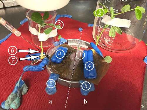
Figure 8. Control examples. Figure 8a illustrates an agar touch performed on Side A. Figure 8b provides an example of an agar touch on Side B. Figure 8c is an example of not receiving a signal after a leaf bend. The arrows indicate the moment of induction.

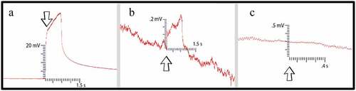
Figure 9. Wound responses conducted across the bridge for cucumber trials 1 and 2.This figure depicts the electrical responses that were conducted from one cucumber plant to another via rhyzoelectric pathways for the six setups. The scale values on the x-axis are in seconds and the scale values on the y-axis are in millivolts. The arrows indicate the moment of induction.

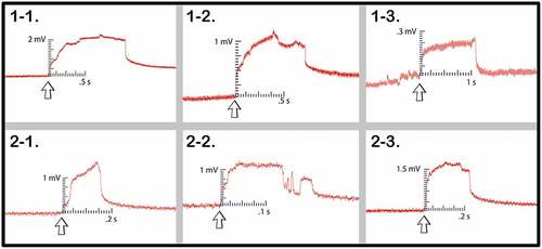
Table 1. This table depicts the magnitude and duration of the wound responses conducted from side B to side A for cucumber trials 1 and 2.

Figure 10. Pea trial 1 signal propagations. This figure depicts the 5 electrical responses that were recorded from one pea plant to another via rhyzoelectric pathways. The scale values on the x-axis are in seconds and the scale values on the y-axis are in millivolts. In setup 4, the change in electric potential and duration of smaller response was used in the table as this was the initial response. The arrows indicate the moment of induction.

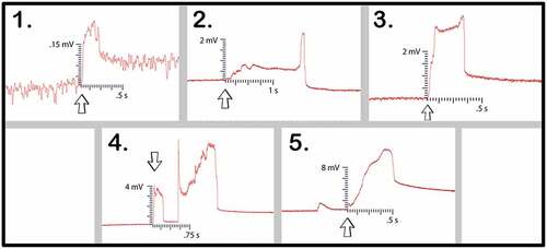
Table 2. This table depicts the magnitude and duration of the wound responses conducted from Side B to Side A for Pea Trial 1.

Figure 11. Pea trial 2 signal propagations. This figure depicts the electrical responses from the four setups in which a successful signal conduction occurred from one plant to another. The scale values on the x-axis are in seconds and the scale values on the y-axis are in millivolts. The arrows indicate the moment of induction.

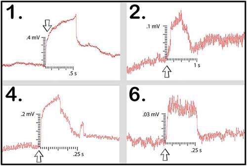
Table 3. This table depicts the magnitude and duration of the wound responses conducted from Side B to Side A for Pea Trial 2.

Figure 12. Pea trial 3 signal propagations. This figure depicts the electrical responses from seven setups which all produced successful signal conductions from one plant to another. The scale values on the x-axis are in seconds and the scale values on the y-axis are in millivolts. The arrows indicate the moment of induction.In the second trial using these direct inoculation methods, all three of the setups successfully conducted electric signals across their respective mycelial bridges. Upon cutting the bridges, the signals could not be conducted from the plant on Side B to the recording electrode in the plant on (Figure 13) and the magnitude and duration of these responses are listed in Table 5.

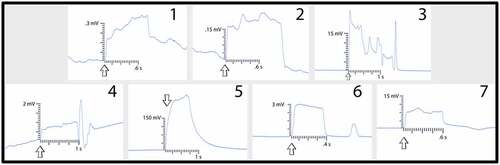
Figure 13. Pea trial 4 signal propagations. This figure depicts the electrical responses from three setups that all produced successful signal conductions from one plant to another. The scale values on the x-axis are in seconds and the scale values on the y-axis are in millivolts. The arrows indicate the moment of induction.

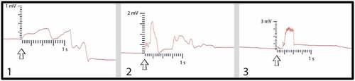
Table 4. This table depicts the magnitude and duration of the wound responses conducted from Side B to Side A for Pea Trial 3. For complex responses, the area under the curve was taken to average the magnitude of the response.

Figure 14. Suture thread electric potentials. This figure depicts the three responses conducted from one plant to another with the moist suture thread bridging the gap. The arrows indicate the moment of signal induction.

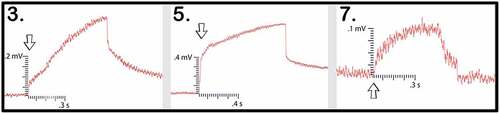
Table 5. This table depicts the magnitude and duration of the wound responses conducted from Side B to Side A for Pea Trial 4. For complex responses, the area under the curve was taken to average the magnitude of the response.

Table 6. This table depicts the magnitude and duration from wound responses on Side A for Cucumber Trials 1 and 2.

Table 7. This table depicts the magnitude and duration from wound responses on Side A for Pea Trial 1. Values of N/A represent those trials in which the signal saturated the recording window.

Table 8. This table depicts the magnitude and duration from wound responses on Side A for Pea Trial 1. Values of N/A represent those trials in which the signal saturated the recording window.

Table 9. This table depicts the magnitude and duration from wound responses on Side A for Pea Trial 3.

Table 10. This table depicts the magnitude and duration from wound responses on Side A for Pea Trial 4.