Figures & data
Figure 1 A simple geometry for a single beam optical trap showing the collimated input laser beam, high NA oil-immersion microscope objective and trapped particle suspended in an aqueous solution. (Figure is provided in color online.).
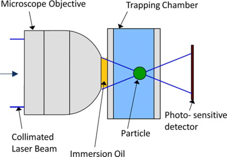
Figure 2 A generic astrophysical AO system utilizing a DM and wavefront sensor. (Figure is provided in color online.).
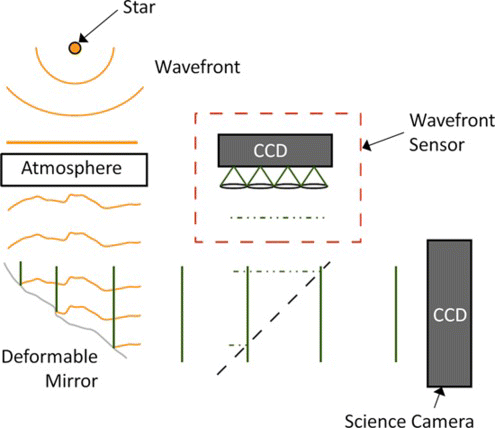
Figure 3 An electromagnetic-based deformable mirror where the actuators are formed by small magnets and micro DC voice coils: (a) Current in each coil creates an electromagnetic attraction/repulsion with the corresponding magnet. (b) Several of the total (52) actuators are outside of the pupil to minimize the effect of the restrained edge. (Figure is provided in color online.).
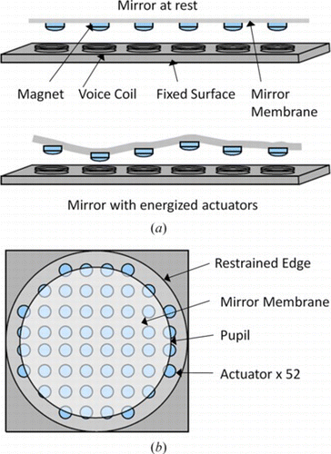
Table 1.
Figure 4 The Shack–Hartmann wavefront sensor measures phase gradient: (a) In the one dimensional sense, the beam phase is sampled by a grid of micro lenses, called a lenslet array, each focusing onto a region of the CCD called a subaperture. (b) The focal point displacement (Δx, Δy) is related to average phase gradient (slope) within the respective subaperture. (Figure is provided in color online.).
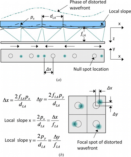
Figure 5 The first five Zernike modes displayed by radial order and physical description (e.g., focus and coma). (Figure is provided in color online.).
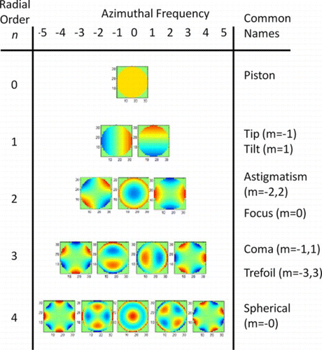
Figure 6 An example of how the tip/tilt mode is created on the DM, and the resulting response from the SHWFS and the trapped bead. The surface of the DM, lenslet array and the back aperture of the microscope objective are all conjugate. (Figure is provided in color online.).
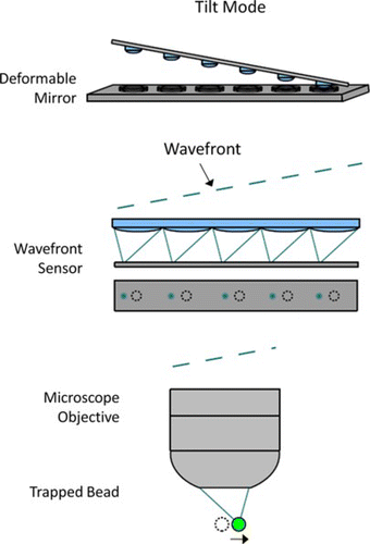
Figure 7 Schematic diagram of the prototype optical trapping system. The lens pairs (e.g., L1, L2) act to resize the beam diameter to fit the pupil of the DM, SHWFS, imaging camera, and back aperture of the trapping objective O1. (Figure is provided in color online.).
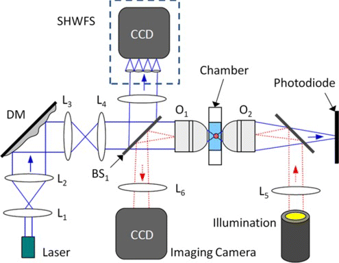
Figure 8 Photograph of the trapping chamber region showing the microscope objectives and cover slips. (Figure is provided in color online.).

Figure 9 (a) Construction of the trapping chamber from two 0.17 mm thick microscope cover slips and a layer of Parafilm. (b) Spatial coordinate system within the trapping chamber. (Figure is provided in color online.).
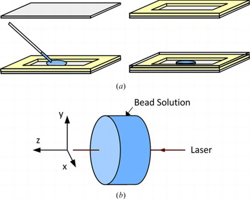
Figure 10 The control system block diagram illustrating how a desired trap location is converted into DM command voltages. The DM and WFS are modeled as single delays Z-1, in control terms. (Figure is provided in color online.).
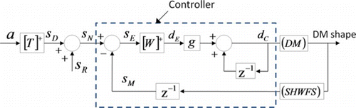
Figure 11 Schematic of the controller parameters as they relate to the SHWFS spots on the CCD. Each spot is moved, in a series of increments, to a desired position based on the required bead location. (Figure is provided in color online.).
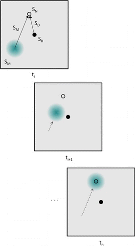
Figure 12 (a) Zernike mode representation of the static wavefront error of the optical system. (b) Zernike representation of the wavefront error with the AO controller activated. (Figure is provided in color online.).
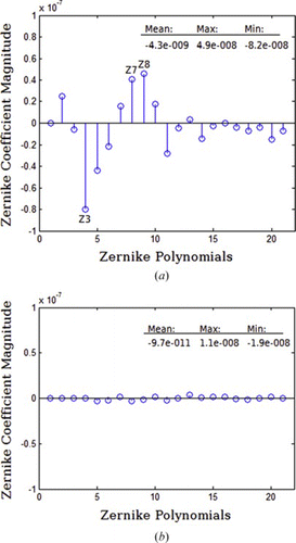
Figure 13 Light focused using an oil-immersion microscope objective is refracted by the oil-solution interface causing spherical aberrations which degrade trap stiffness: (a) shows a tight focus close to the cover slip and (b) shows an extended focus at increased depth, degrading the trap stiffness. (Figure is provided in color online.).
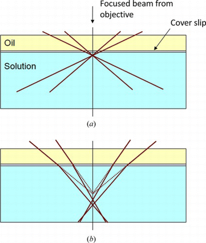
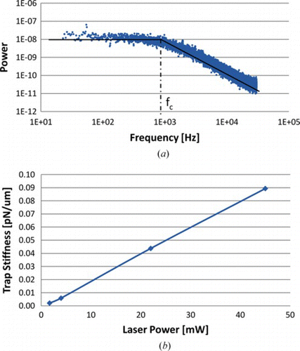
Figure 14 (a) Power spectral density measurement of a single trapped particle for a laser power of 10 mW measured at the entrance to the microscope objective. (b) Trap stiffness for different laser powers. The average error in the stiffness was estimated to be 10% of the displayed values. (Figure is provided in color online.).