Figures & data
Figure 1 The errors of tomographic reconstruction using Hybrid FBPJ and FBPP for fiber having step-index profile.
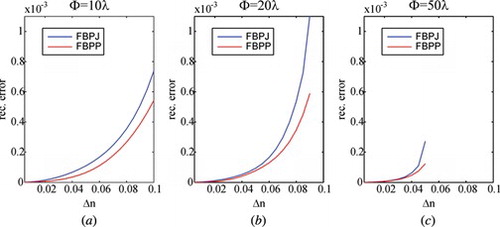
Figure 2 Measurement setup for full angle (a) and limited angle tomography module (b). Figure 2(a): SMF—single mode fiber, light source—frequency doubled Nd:YAG laser λ = 532 nm; CL—collimating lens (f’ = 50 mm); BS1, BS2—50:50 Beam splitting cube; M1, M2—mirror; PD—Petri Dish; FC—Fiber capillary; MO—Long working distance 20x microscope objective; TL—Tube lens (f’ = 150 mm); CCD—Charge-Coupled Device camera. Figure 2(b): MRM—Motorized rotary mirror; TL1—tube lens (f’ = 75 mm); BFP—back focal plane; SPL—specimen plane; TL2—tube lens (f’ = 150 mm).
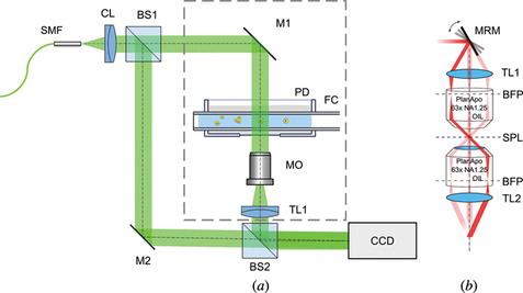
Figure 3 The self-interference Digital Holographic Microscope with the rotary fiber holder setup. WL—white light source, SMF—single mode fiber, CL—condenser lens, BS—beamsplitter, PD—Petri dish, IL—immersion liquid, FC—fiber capillary, MO—microscopic objective, M—mirrors.
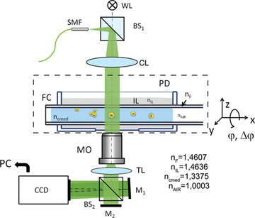
Figure 4 The flow chart of the tomographic procedure from capture to 3-D refractive index determination.
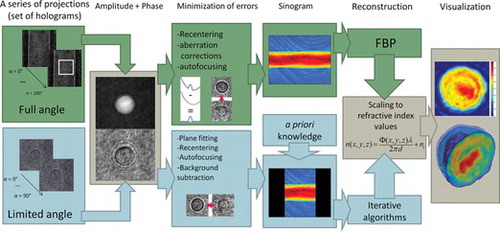
Figure 5 The correction of phase aberration associated with the fiber capillary: (a) original phase distribution; (b) cross-section of the phase distribution (solid line) and of the fitted aberration profile (dashed line); (c) and (d) the correction results.
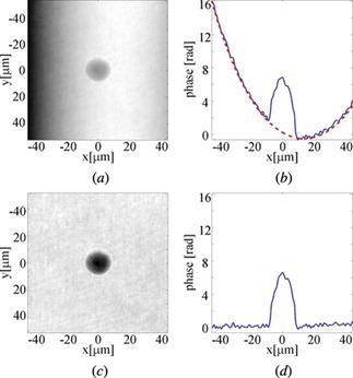
Figure 6 The examplary results of 3-D refractive index distribution in (a) cluster of HT1080 cells and (b) horizontal and (c) vertical cross-section of HT1080 cell with an extension, (d) horizontal and (e) vertical cross-section of U937 human malignant lymphoma cell.
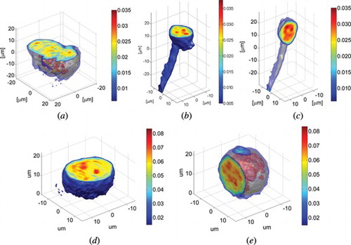
Figure 7 The reconstruction of a middle layer of U937 cell (a) from the projections captured from a full angular range (reference image), (b) from the projections taken within 90° with Filtered Back Projection algorithm (c) from the projections taken within 90° with DRA with additional geometry mask (after 13 iterations) and (d) the error calculated after each iteration between the reconstruction and reference image for 30 iterations.
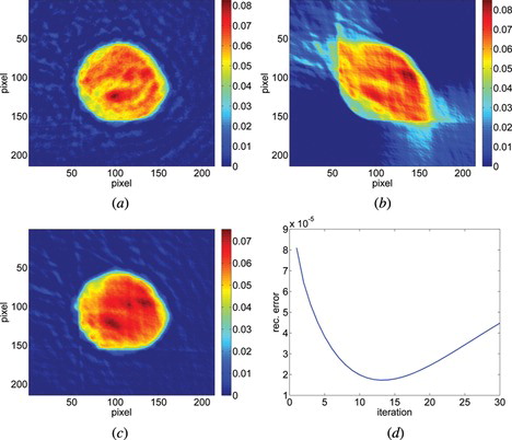
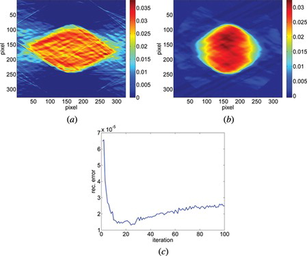
Figure 8 The reconstruction of a middle layer of polymer microsphere (a) from the projections taken within 80° with Filtered Back Projection algorithm (b) from the projections taken within 80° with SART + TVM (after 22 iterations) and (c) the error calculated after each iteration between the reconstruction and reference image for 100 iterations.